(日本語による解説はここをクリック）

The explanation of the DSMC method in Section 5.1 was compiled during my employment as a university educational material and a subcommittee material for academic societies, and similar content is also published in the Computational Mechanics Handbook III (Reference 3) compiled by the Japan Society of Mechanical Engineers. More than 20 years have passed since the first material was distributed, so it is not up-to-date, but it contains many of the points necessary to understand the content that appears on this website (blog). Although some parts have been revised from the original description, it is mainly based on the books (References 1, 2) and papers (References 12, 13, 14) by Bird, the founder of the DSMC method, so this section does not mention U_system or program parallelization.

Basics of the DSMC method

1. Introduction

The direct simulation Monte Carlo method (DSMC method) was developed by Bird in 1963 as a numerical calculation method for rarefied gas flows. The position coordinates and velocity components of many molecules are stored in the computer, and the “spatial movement” and “intermolecular collisions” of these molecules are separated in small time steps (uncoupling of molecular spatial movement and intermolecular collisions), and the flow field is analyzed by repeating the calculations alternately. This method became widely known around the world with the publication of Bird’s book on the DSMC method in 1976 (Reference 1), and a revised and significantly revised version was published in 1994 (Reference 2). During that time, molecular and collision models have made great advances, and coupled with advances in computer technology, it has become possible to use this method in a wide range of fields, from molecular flows to continuum flows, as well as in three-dimensional analysis. Furthermore, there have been attempts to apply this method, taking advantage of its microscopic analysis characteristics, to the analysis of unstable fluid phenomena (see Chapters 3 and 4 of this website). Here, in order to explain the basics of the DSMC method, we will take up a “supersonic rarefied free jet in an axisymmetric field” as an example and look at the details of the DSMC method while referring to its Fortran program (simplified version). Fortran has a very small number of instructions (only seven statements need to be understood: variable types, input/output statements, assignment statements, block IF statements, DO loops, GOTO statements, and subprograms; it is similar to VBA language, but calculations are fast because it is basically a compiler system) and even beginners can learn it in a relatively short time, so it is effective for understanding the DSMC method. In the DSMC method, many parts of the program can be used in common regardless of the problem being addressed, so we believe that the example problem in this section can be used as a core to apply it to various flow fields. It is also possible to develop this example problem from monatomic gases to diatomic or polyatomic gases, from simple gases to mixed gases, and even flows that include chemical reactions. We will look at the details in order, but first we will list the outline of the calculation procedure of the DSMC method and its features.

2. Overview of the calculation procedure of the DSMC method

[1] First, a molecule is given initial coordinates and initial velocity components by random numbers and placed in the target physical space. The physical space is divided into tiny spaces called cells. Ideally, the size of one side of a cell should be smaller than the local mean free path.

[2] The calculation of the movement of molecules in physical space (including collisions with solid walls and entry and exit at inflow and outflow boundaries) and the calculation of intermolecular collisions are separated by an infinitesimal time step $\mathrm{\Delta }t$ (ideally smaller than the local mean collision time) and are calculated independently (uncoupling of molecular spatial movement and intermolecular collisions). In other words, the following three-step process is repeated.

(a) Each molecule moves through space independently of other molecules for a time $\mathrm{\Delta }t$ according to its speed. If a molecule reflects off a wall surface or flows out from a boundary, the momentum and energy flow is calculated. Also, new molecules flow in from the boundary.

(b) Since the position coordinates of each molecule change due to molecular movement, the cell to which the molecule belongs is investigated, and all molecules are rearranged in the “cross-reference array” in preparation for intermolecular collisions. In other words, each cell is given a consecutive number (seat number) equal to the number of molecules present in it as an array subscript, and the molecular number is stored in the array element. In collision calculations, once a seat number belonging to a cell is determined, this array is used to cross-reference the molecular number from the seat number, and information such as the molecular velocity components can be extracted.

(c) Intermolecular collisions are calculated for each cell based on the collision law. The main content is to calculate the number of collisions that occur within $\mathrm{\Delta }t$ time, select collision pairs, and determine the velocity components after the collision. Note that the collision calculation does not take into account the molecular position within the cell. On the other hand, in the U_system as will be explained in Section 5.2, corrections are made to the molecular velocity before and after the collision depending on the molecule’s position within the cell, so the cell can be made larger.

[3]The above steps (a) to (c) are repeated, and the ensemble average of the flow field quantities is calculated for unsteady problems, and the time average after the steady state is achieved is calculated for steady problems. Note that ensemble averaging is performed to compensate for the small number of molecules per cell, but if you average cells in a range with little spatial change, or take a time average of a range with little temporal change, it is possible to perform an unsteady analysis without performing ensemble averaging. The animations shown in Sections 3.1 and 4.2 were obtained in this way.

3. Characteristics of the DSMC method (advantages and disadvantages)

[1] The calculation is based on the motion of individual molecules, so it has the disadvantage of taking a huge amount of time. DSMC is good at rarefied gases and high-speed gases, but when the density is high (even if high it is below 1 atmosphere) or when the speed is low, it takes a long time to reach a steady state, making the analysis more difficult. When the most probable molecular thermal speed is 350 m/s, the flow is analyzed based on that molecular motion, so in order to keep the statistical fluctuation of the results low, a significant number of sample molecules (or calculation repetitions) are required to clarify a phenomenon at a low speed, such as 1 m/s. However, if the analysis target is not the flow speed, it is possible to analyze even a stationary gas.

[2] Boundary conditions are easy to set. For example, it is only necessary to set the molecular reflection law at a solid wall, and in engineering calculations, simple diffuse reflection (scattered reflection) is often sufficient. The calculation of the inflow position and velocity components of molecules at the inflow boundary, or the number of inflow molecules, can also be easily determined according to the macroscopic state quantity. In the DSMC method, the conditions given to the inflow and outflow boundaries are applied only to molecules flowing in from the boundary, and are not directly applied to molecules flowing out of the calculation domain (of course, they are indirectly affected by collisions with molecules flowing in from the boundary). Therefore, even if an extreme state such as infinite distance is given to the boundary condition, the outflowing molecules are not strictly bound by it, and the calculation does not diverge. Of course, it is preferable for the boundary conditions to be such that there is no difference in the macroscopic state of the inflowing and outflowing molecules, so a method for achieving this is important. Note that if there is a difference between the two, distortion will occur in the flow field near the boundary, but this does not mean that the results for the entire domain will be completely meaningless.

[3] The DSMC method is essentially an unsteady calculation because the calculation progresses over time. Therefore, there is no essential difference in the difficulty of calculations between steady and unsteady problems. This means that even if it is a problem for solving a steady condition, a solution cannot be obtained unless an unsteady state has passed.

[4] Cell division (grid cutting) of the flow field is easy. Since the spatial movement of molecules is performed regardless of the cell structure, it is not necessarily necessary to divide the cells along the boundary shape (details will be described later).

[5] The main part of creating a new program is the routine for cell division and molecular movement. Existing routines can be used for the part related to intermolecular collisions. However, creating a program for molecular movement is extremely difficult without experience.

[6] It can be used to analyze not only rarefied gas flows but also micro flows. The DSMC method was developed as a numerical analysis method for rarefied gas flows. As shown in the example, it is now used in regions where the state changes significantly, from molecular flow to continuous flow, and in the future, it will be improved so that it can be applied to flows at atmospheric pressure. On the other hand, in the world of micro flows, the DSMC method can be used as is even at atmospheric pressure. The dimensionless number that represents the degree of rarefaction is the Knudsen number $K_n$, which is defined as follows using the mean free path $\lambda$ and the characteristic length $L$.
$$\begin{array}{}\text{(1)}& K_n=\lambda /L\end{array}$$The larger $K_n$, the greater the rarefaction, making it easier to analyze with the DSMC method. Rarefied gas generally refers to a state with low density, that is, a state where $\lambda$ is large, but even if $\lambda$ is small, $K_n$ increases if $L$ is smaller than that. This is a micro flow.

4. Outline of the example

To explain the basics of the DSMC method, we will take up the example of “supersonic rarefied free jet in an axisymmetric field” and proceed with the explanation while referring to a Fortran program (Click here to see the program list). Note that the one to three digits and one space following each number on the left side of each line in the program indicate the line number (1 to 677) and are not included in the program. In the text, when describing variables in the Fortran program, we will underline the variable symbols to avoid misunderstandings (for example, TEMP). The example is a very simplified program of about 700 lines, but it has almost all the basic features. As shown in Figure 1, in a simple flow field consisting of a zero-thickness wall with a circular orifice of radius EZA (actual radius is 0.00125 m) and the space (computational space) that spreads to the right of it, the flow field is surrounded by inflow and outflow boundaries (boundaries with a density equivalent to the downstream back pressure, hereafter referred to as downstream boundaries) except for the orifice wall (circular aperture and wall surface). The downstream boundary can be divided into a boundary parallel to the central axis (peripheral boundary) and a boundary perpendicular to the central axis (vertical boundary), but when simply called downstream boundary, it refers to both.

Since the field is axisymmetric, the calculation space is represented only above the central axis (the central axis of the jet). The cell division is two-dimensional, but the flow field has a three-dimensional spread. The flow velocity is assumed to be uniform and equal to the speed of sound ($M=1$) at the orifice cross section, and the density and temperature are determined assuming that the flow reaches the orifice aperture from the upstream stagnation point due to an isentropic change. The macroscopic flow velocity at the downstream peripheral boundary is assumed to be zero, and the macroscopic flow velocity at the downstream vertical boundary is determined by averaging the velocity of the molecules near the boundary, which changes as the calculation progresses. In addition, the molecules are diffusely reflected at the orifice wall. The gas is assumed to be a single gas of monatomic argon. The initial density of the flow field is set to be equal to the value at the downstream boundary, and the simulation is performed from time zero, when gas flows in through the orifice aperture, until the formation of a supersonic jet. In this program, numerical values ​​for all variables are given in SI units. The pressure at the upstream stagnation point is 6700 Pa (50 Torr), the downstream back pressure is 1/50 of that (1 Torr), and the temperature is both 15°C. In order to accurately reproduce the jet structure, it is necessary to provide a calculation space upstream of the orifice, but this is omitted in this simple program.

5. Generation of random numbers from a prescribed distribution

Here, we will introduce three methods for creating random numbers from a prescribed distribution required for DSMC calculations using real random numbers (hereafter referred to as uniform random numbers $R_f$) that are uniformly distributed from 0.0 to 1.0.

[1] Inverse transform method (Direct method)

When the value $A$ is obtained by integrating a specific distribution function $f_0$ over the entire valid area (all intervals $a$ to $b$), the distribution function $f$ obtained by dividing the distribution function $f_0$ by $A$ is called a normalized distribution function (it can also be considered as a distribution function that becomes 1 when integrated over the entire area).
$$\begin{array}{}\text{(2)}& f=f_0/A, A={\int }_a^b{f}_{0}dx\end{array}$$Furthermore, the integral of $f$ from $a$ to an arbitrary value $x$ is called the cumulative distribution function $F_x$.
$$\begin{array}{}\text{(3)}& F_x={\int }_a^{x}fdx\end{array}$$If we equate the cumulative distribution function $F_x$ to $R_f$ and can solve it explicitly for $x$, that is, if we can write $x=g(R_f)$ and calculate $x$ from $R_f$, then we have obtained a random number $x$ that follows a specific distribution $f_0$ from the uniform random number $R_f$. For example, if we assume that molecules are uniformly distributed within a circle of radius $r_0$ and we wish to find the distance $r$ from the center of the circle of one of those molecules (this corresponds to finding the position coordinate $y$ of a molecule flowing in from an orifice aperture, and generating a molecule on the downstream boundary perpendicular to the central axis, in the example problem in this section), the probability of that molecular position is proportional to $r$, so we can find the cumulative distribution function as follows.
$$\begin{array}{}\text{(4)}& F_r={\int }_0^{r}2r/r_0^{2}dr=r^2/r_0^2\end{array}$$ If we solve this by equating it to the uniform random number $R_f$, we obtain the following equation.
$$\begin{array}{}\text{(5)}& r=r_0\sqrt{R_f}\end{array}$$
<Assignment> When molecules are uniformly distributed inside a spherical shell with an inner sphere of radius $a$ and an outer sphere of radius $b$, generate the distance of one molecule from the center of the sphere.

[2] Acceptance-rejection method

The inverse transform method mentioned above cannot be used unless the equation connecting the cumulative distribution function $F_x$ and $R_f$ with an equal sign can be explicitly solved. In contrast, as shown in Figure 2, by enclosing any distribution function in a rectangle and finding one random number for each of the width $X$ and height $Y$ of the rectangle, a random value that follows the distribution function can be generated. In other words, a point is determined within the rectangle using two random numbers, and if that point is below the distribution function (within the distribution), the value $x_1$ at that point becomes the desired value. If the point falls outside the distribution, random numbers are generated again horizontally and vertically to find one more point, and this is repeated until the point falls within the distribution. This method can be applied to any distribution, but it is necessary to use two or more uniform random numbers to find one value. In particular, the efficiency decreases as the area inside the distribution function becomes smaller compared to the area of ​​the rectangle. Therefore, for distributions such as the equilibrium velocity distribution function of molecules, which theoretically have infinite velocities but the probability approaches zero as the velocity increases, it is necessary to set a cutoff value to limit the width. In the example problem in this section, this method is used to generate the velocity components perpendicular to the orifice surface of the molecules flowout through the orifice. The details will be explained later.

[3] A method to simultaneously obtain two normally distributed values

There is an efficient method to simultaneously obtain two normally distributed values, such as thermal velocity components in an equilibrium gas. Let $f_{u^{\prime }}$ be the distribution function of the velocity component $u^{\prime }$ in the $x$ direction (the $x$ component of the thermal velocity obtained by subtracting the macroscopic flow velocity from the actual velocity of the molecules) in the equilibrium condition, and $f_{v^{\prime }}$ be the distribution function in the $y$ direction.

$$\begin{array}{}\text{(6)}& f_{u^{\prime }}=\frac{\beta }{\sqrt{\pi }}\exp (-{\beta }^2{u}^{\prime 2}), f_{v^{\prime }}=\frac{\beta }{\sqrt{\pi }}\exp (-{\beta }^2{v}^{\prime 2})\end{array}$$ Here, $\beta$ is the inverse of the most probable molecular thermal speed $c_{max}^{\prime }(=\sqrt{2RT})$, $R$ is the gas constant, and $T$ is the absolute temperature. These velocity distribution functions are normalized. Multiplying the two distribution functions give $$\begin{array}{}\text{(7)}& f_{u^{\prime }}d{u}^{\prime }\times f_{v^{\prime }}d{v}^{\prime }=\frac{{\beta }^2}{\pi }\exp \{-{\beta }^2(u^{\prime 2}+v^{\prime 2})\}d{u}^{\prime }d{v}^{\prime }\end{array}$$

Now, if we replace the variables $u^{\prime },v^{\prime }$ with $r,\theta$ as follows:
$$\begin{array}{}\text{(8)}& u^{\prime }=r\cos \theta ,v^{\prime }=r\sin \theta \end{array}$$

$$\begin{array}{}\text{(9)}& f_{r}dr{f}_{\theta }d\theta =\frac{{\beta }^2}{\pi }\exp (-{\beta }^2{r}^2)rdrd\theta =\frac{1}{2\pi }\exp (-{\beta }^2{r}^2)d({\beta }^2{r}^2)d\theta \end{array}$$

Therefore, $f_{\theta }=$Const., $f_{{\beta }^2{r}^2}=$Const.$\times \exp (-{\beta }^2{r}^2)$, and the integral ranges are $\theta =0\sim 2\pi$, ${\beta }^2{r}^2=0\sim \mathrm{\infty }$. Now, if we apply the inverse transform method described above to the two, we get
$$\begin{array}{}\text{(10)}& \theta =2\pi R_{f1}\end{array}$$

$$\begin{array}{}\text{(11)}& r=\sqrt{-{\log }_e(1-R_{f2})}/\beta \end{array}$$

However, because $R_{f2}$ and $1-R_{f2}$ are the same due to the nature of uniform random numbers,

$$\begin{array}{}\text{(12)}& r=\sqrt{-{\log }_e{R}_{f2}}/\beta =\sqrt{-2RT{\log }_e{R}_{f2}}\end{array}$$
That is, the velocity components $u^{\prime },v^{\prime }$ can be calculated simultaneously from two different uniform random numbers $R_{f1}$ and $R_{f2}$ using equations (8), (10), and (12). This molecular velocity generation equation in equilibrium can also be applied to calculate the velocity components parallel to the wall when the molecules are diffusely reflected on the wall. Of course, in that case, the value equivalent to the wall temperature is used for $\beta =1/\sqrt{2RT}$.

6. Function subprogram

In addition to the main program, the example program has three subprograms at the beginning. The first, RANF0(), is a function that generates uniform random numbers using the congruential method, and has a period of $2^{29}$. The initial value of the integer random number that is the source of this random number is the value of IRAN on line 52 of the example program (in the following descriptions, “line xxx” is refer to a line number in the example program), and this value can be any odd number. If you want to change the initial random number, replace this with any odd number. If there is another reliable uniform random number routine, you can use it, or if possible, it is preferable to use long-period random numbers using 64-bit integers.

The second subprogram, GAM(X), calculates the gamma function, and performs an approximation using Chebyshev’s series. This is used in the calculation of the VHS and VSS molecular models. The third subprogram, ERF(X), calculates the error function, and is used to calculate the number of inflowing molecules when there is a macroscopic flow rate at the inlet of the molecules. In the example, it is used to calculate the number of inflowing molecules from the orifice aperture. The formula for this error function uses the formula by Abramowitz et al.

7. Array variables used in DSMC calculations

The real variables used in the DSMC method are basically double-precision real numbers (see IMPLICIT statement). This is to minimize errors in the spatial movement of molecules. However, since the arrays for storing information on molecules or cells are large, single-precision real numbers are used for these large arrays in the example (if the PC has sufficient memory, it is better to use double-precision arrays as they are). In other words, the molecular velocity component P(3,MOL), the position coordinates PZ1(MOL) and PZ2(MOL), and the cell volume CTA(NCELL). Note that MOL is the maximum number of molecules, and NCELL is the maximum number of cells. By changing the values ​​in the PARAMETER statement according to the capacity of the computer, it is possible to handle even larger numbers of molecules and cells. LCR stores the cross-reference array used in intermolecular collision calculations, and IP stores the cell number to which the molecule belongs. Note that since the example is an axisymmetric calculation, the $z$ coordinate PZ3 is not necessary, but it is necessary for three-dimensional calculations. IC1 stores the number of molecules in the cell, and IC2 stores the first address of each cell in the cross-reference array minus one (first address $-1$) (details will be described later). In this program, the coordinates of the cell center are not stored as array variables, but are calculated on the spot when necessary. In addition, when it comes to three-dimensional problems, the number of cells increases dramatically, so the number of molecules in the cell must be reduced. However, if the number is within 127, IC1 can be made a one-byte integer to save memory. SC(8,NCELL) is an array that stores the raw information used to calculate the macroscopic physical quantities of each cell (sample cell). In this example, the same cell as the collision cell for intermolecular collisions is used for also data sampling, but if the number of collision cells becomes large, several collision cells can be combined into a sample cell to save this array. SS stores the number of molecules flowing in and out of the boundary. In addition, variables that store the momentum and energy balance when reflected from the wall are generally used, but they are not used in this example. OP and ASC are work arrays, a series of string variables are used to store file names for outputting results, PRI is an array to store flow rates (dimensionless conductance) at the boundaries, and U0 is an estimate of the flow velocity at the downstream vertical boundary.

8. Starting the example (supersonic free jet) program

IERRx is a counter to check the number of errors during calculation, RVRALL and RVRGT are variables to check the maximum number of collisions in intermolecular collisions, IRAN is a random integer number (odd number), and PI is the circular constant.

The upstream stagnation point temperature TEMP and the orifice wall temperature TEMPW are 15[°C] (288[K]), the upstream stagnation point pressure PTOR is 50[Torr], PPAS is the pressure in [Pa], ANUM is the number density $n$ in [1/m${}^3$], and PRAT is the ratio (pressure ratio) of the upstream stagnation pressure to the downstream back pressure, which is 50. The orifice diameter ORID is 0.0025[m].

In the DSMC method, molecular movement and intermolecular collisions are separated (uncoupled) at a time step $\mathrm{\Delta }t$ and the calculation is repeated. After this is repeated NIS times, the raw information of the cell is sampled. This is one RUN. However, NIS in this case is 1. After one RUN is repeated K100 (=5000) times, the raw information in the cell is averaged and output to a file. The first four characters of the output file name are ‘sjet’. I9 is ​​the number of RUNs for calculation termination, and in this case the calculation will end at 100000 times. In other words, 20 output files are created.

9. Cell division of the flow field

The cells that divide the flow field have two roles. One is that intermolecular collisions occur between molecules in the same cell, and the other is that the cells are used as infinitesimal elements to sample flow field information such as density, velocity, and temperature. Since molecules in the same cell are subjected to collision calculations regardless of their relative positions, ideally the length of one side of a cell should be smaller than the local mean free path. However, in axisymmetric or three-dimensional problems, it is difficult to make the cell length less than the mean free path when the size of the flow field and its density become large, and it is sometimes unavoidable to make the cells larger due to limitations in computer capacity. However, even if the cells are made larger, the results obtained do not become completely unreliable; the change rates of physical quantities such as density and temperature simply appear somewhat more relaxed than they should be. Therefore, cells can be made larger in places where the state changes are gradual, while if cells are made larger in places where the change is steep, results that are somewhat more relaxed than the original changes can be obtained. Keep this in mind when using the DSMC method. The simplest method of cell division is to divide the space into rectangular cells. Cell division can be done rectangularly even if the boundary is an arbitrary curved surface. This is because the cells are not involved in the spatial movement of molecules at all, and even in a rectangular cell structure, molecular movement is consistent with the boundary shape (the volume of the space in which the gas actually exists must be calculated). In the case of a complex boundary shape, some cells may become extremely small in volume, causing concern that there will be almost no molecules in the cell and causing problems in collision calculations. However, this effect will not be apparent unless a considerable number of nearby cells become small collectively.
Bird (Reference 12) devised the subcell division method in 1987 when comparing calculation methods with the molecular dynamics method (MD method) for vortex generation. The time counter method (TC method), which was the mainstream intermolecular collision methods at the time, required more than 20 molecules to be contained in a cell, so in order to ensure this number and keep the distance between colliding molecules below the mean free path, the normal cell grid was divided into even finer cells. However, in the currently commonly used maximum collision number method (null collision method, no-time-counter method), the theoretical collision number is satisfied even if the number of molecules in the cell is about one (Reference 15), so the role of the subcell method is not as important as it was originally. In addition, the program code of the subcell method shown in Bird’s book (Reference 2) was created for one-dimensional calculations, so it does not necessarily provide accurate calculations when applied to two- or three-dimensional problems. Recently, Usami et al. (References 3, 4, 5) developed a method called the U-system to calculate collisions taking into account the molecular positions within the cell. The details of this method, which gives very good results even if the cells are much larger than the mean free path, are explained in Section 5.2.

The density of the free jet in the example drops rapidly as it moves downstream, so the cell structure (axial cell division) that subdivides the flow field is designed to increase the cell length in a geometric progression as it moves downstream, so that there is no large difference in the number of molecules in each cell. Now, on the central axis, the axial length of the cell immediately after the orifice is $a$ (Fortran variable is TKN), the common ratio is $b$ (ES0), and the length of the $i$th cell is $a{b}^{i-1}$. In this case, if the coordinate of a molecule is $x$, the axial number $j$ of the cell to which the molecule belongs can be easily calculated as follows (Reference 16).
$$\begin{array}{}\text{(13)}& j=\frac{\log \{x(b-1)/a+1\}}{\log b}+1[decimal.parts.are.truncated]\end{array}$$

In this case, the number of cells in the axial direction KS is 164, and the common ratio ES0 is 1.02. On the other hand, the radial cell division is basically first divided equally into 40 cells (I2) of length TKN for the orifice radius EZA, and the entire radial cell structure of the flow field is also divided equally, with the number of divisions KO being 240. AL1 and AL2 in lines 82-83 are $(b-1)/a$ and $1/\log b$ in equation (13).

If the radial direction is divided equally in an axisymmetric field, the cell volume on the central axis becomes extremely small and a sufficient number of molecules cannot be secured. Therefore, in the example, only the cells on the central axis are operated to combine three adjacent cells in the radial direction to form one cell.

The cell volume CTA is calculated in the double DO loop in lines 87-104. Because of the axisymmetric flow field, the cells other than those on the central axis have a ring structure. The three cells closest to the central axis are combined to form one, making this a somewhat complicated routine. Additionally, the total number of cells, NC, is KS$\ast$(KO$-$2). Note that although the three cells on the central axis are connected, the cell on the central axis just after the orifice before they are connected is used as the “reference cell”. The weighting factor of the simulation molecules (described later) and other factors are explained using this reference cell. The volume of the reference cell is specifically stored as CH,and is TKN$\ast$TKN$\ast$TKN$\ast$PI (line 109).

<Assignment> A plate with zero thickness is placed diagonally in a flow field divided into a grid of rectangular cells, and some cells are divided into the front and back of the plate. In such a case, consider how to handle the cells divided by the plate.

10. Number of molecules in a cell and weighting factor of simulated molecules

The number of molecules in a gas is $6\times {10}^{23}$ per mole, and even in a very dilute state, it is difficult to move the same number of molecules as in a real gas in a computer. On the other hand, the DSMC method is a statistical calculation. Even without analyzing the motion of all molecules, a part of them is extracted (sampled) and the motion of the entire molecule is predicted. For example, if a certain location (cell) in the flow field is analyzed using the average value of 1 million sample molecules, reliable results can be obtained with an error of about $\pm 0.1$%. Now, regarding these 1 million sample molecules, in the case of a zero-dimensional problem, one cell is sufficient and calculations can be performed without any problems, but in a three-dimensional problem with, say, 1 million cells, the total number would be ${10}^{12}$, which is extremely difficult with the computer systems available to the author. Therefore, for example, one calculation can be performed by putting 10 molecules into a cell and analyzing it, and repeating the same calculation 100,000 times, thereby securing 1 million sample molecules. So, what is the number of molecules in a cell in one calculation? This depends on the problem, so it cannot be said in general, but in the case of the supersonic free jet shown in the example, it has been reported that a reasonable result can be obtained if there is at least one molecule in the cell on a time average (Reference 15). Note that one molecule per cell is an extreme case, and personally, I think that four or more molecules are preferable.

In this way, regardless of the number of molecules in the real gas, the number of molecules in the DSMC method can be determined quite freely, but it is necessary to remember how many real molecules each simulation molecule represents. This is called the weighting factor WEI. In other words, in calculating the number of intermolecular collisions per time step $\mathrm{\Delta }t$, the apparent collision cross section ${\sigma }_T$ must increase in inverse proportion to the decrease in the number of molecules, and this weighting factor is used to correct it. Note that it is not correct to think that “the simulation molecules themselves become larger, and a giant molecule that is a group of a number equivalent to the weighting factor moves in the calculation space.” The simulated molecules are sampled (sampling) from a large number of real molecules, and should be considered to have the same size and mass as the real molecules.

In the example, the real molecular number density at the upstream stagnation point is ANUM [1/m${}^3$]. Therefore, the number of molecules in the reference cell volume CH is BNUM when the density is the value at the stagnation point (line 110). In the simulation, AMC (=0.5) molecules are placed in this cell (line 75), so the weighting factor WEI is calculated on line 111. Note that although the density is lower immediately after the orifice than at the stagnation point, the number of molecules exceeds 1 because three cells on the central axis are connected.

<Assignment> If the number of molecules in the cell is one in time average, a question arises as to whether a collision partner cannot be found. However, the simulation is valid. Consider this point.

11. Molecular model (VHS molecule and VSS molecule) – collision calculation part 1

One of the significant improvements in the DSMC method is the molecular model. In the early days (Reference 1), hard sphere molecules were used if calculation speed was a priority, and inverse power law molecules were used if faithfulness to real molecules was a priority. Later, Bird analyzed many calculation results and concluded that “the reason inverse power law molecules produce good results is not because they faithfully reproduce the deflection angle in collision calculations, but because the collision cross section is a function of the relative translational energy.” In a 1981 paper (Reference 13), he published the VHS molecular model, which maintains the hard sphere scattering law (in the collision of hard sphere molecules, there is no probabilistically dominant direction for the relative velocity after the collision) and makes the collision cross section a function of the relative velocity (i.e., a molecular model in which the molecular diameter is a function of the relative velocity). This molecular model has excellent calculation speed because it has collision dynamics almost the same as hard spheres, and it also produces calculation results similar to the inverse power law molecule. Now, assuming that the temperature $T_{ref}$ and the viscosity coefficient ${\mu }_{ref}$ are the values ​​in the reference state, the reference diameter of the VHS molecule can be calculated by the following formula.

$$\begin{array}{}\text{(14)}& d_{ref}=\sqrt{\frac{5(\alpha +1)(\alpha +2)(mk{T}_{ref}/\pi {)}^{1/2}}{4\alpha (5-2\omega )(7-2\omega ){\mu }_{ref}}}\end{array}$$

Here, $m$ is the molecular mass, $k$ is the Boltzmann constant, $\omega$ is the temperature exponent of the viscosity coefficient, and $\alpha$ is 1. $\omega$ is determined by experimentally determining the temperature dependence of the viscosity coefficient. Table 1 shows the $\omega$ values ​​for several gases (Reference 2).

Table 1 Temperature exponent of viscosity coefficient ω

$$\begin{array}{}\text{(15)}& {\sigma }_{Tref}=\pi d_{ref}^2\end{array}$$

$$\begin{array}{}\text{(16)}& {\sigma }_T={\sigma }_{Tref}\{2k{T}_{ref}/(m_r{c}_r^2){\}}^{\omega -0.5}/\mathrm{\Gamma }(5/2-\omega )\end{array}$$

Here, $\mathrm{\Gamma }$ is the gamma function.

$$\begin{array}{}\text{(17)}& {\sigma }_T{c}_r={\sigma }_{Tref}\frac{(2k{T}_{ref}/m_r{)}^{\omega -0.5}}{\mathrm{\Gamma }(5/2-\omega )}{c}_r^{2(1-\omega )}\end{array}$$

Furthermore, using the diameter $d_{ref}$ of the VHS molecule, the mean free path $\lambda$ can be calculated as follows:

$$\begin{array}{}\text{(18)}& \lambda =\frac{1}{\sqrt{2}\pi d_{ref}^{2}n(T_{ref}/T{)}^{\omega -0.5}}\end{array}$$
The Knudsen number $K_n$ is calculated from this value of $\lambda$. The collision dynamics of VHS molecules are exactly the same as those of hard spheres. In other words, the absolute value of the relative velocity $c_r$ does not change before and after the collision, and the direction of the relative velocity after the collision has no directivity (no probabilistically dominant direction). Therefore, the direction can be selected so that it is proportional to the solid angle. Now, if we consider the velocity space in polar coordinates, and the polar angle of the velocity vector is $\theta$ and the azimuth angle is $\varphi$, the elements of the solid angle of the polar coordinates are $\sin \theta d\theta d\varphi$. Therefore, the azimuth angle $\varphi$ is uniformly distributed in the range of $0\sim 2\pi$, and the polar angle $\theta$ is distributed in the range of $0\sim \pi$ with the distribution function $f_{\theta }=\sin \theta$. By rearranging this, we obtain the following equation.

$$\begin{array}{}\text{(19)}& f_{\theta }d\theta =\sin \theta d\theta =-d(\cos \theta )=f_{\cos \theta }d(\cos \theta )\end{array}$$

That is, $\cos \theta$ is uniformly distributed in the range of $-1\sim 1$. The three components of the relative velocity after the collision are the absolute value of the relative velocity $c_r$ multiplied by $\cos \theta ,\sin \theta \cos \varphi ,\sin \theta \sin \varphi$, so first calculate $\cos \theta ,\sin \theta$ using uniform random numbers from $-1\sim 1$, then calculate $\varphi$ using uniform random numbers from the range of $0\sim 2\pi$ and calculate $\cos \varphi$ and $\sin \varphi$. To summarize the above, the relative velocity components $u_r^{\ast }$, $v_r^{\ast }$, $w_r^{\ast }$ after the collision can be calculated as follows:


$$\begin{array}{}\text{(20)}& \cos \theta =2R_{f1}-1\end{array}$$

$$\begin{array}{}\text{(21)}& \sin \theta =\sqrt{1-{\cos }^2\theta }\end{array}$$

$$\begin{array}{}\text{(22)}& \varphi =2\pi R_{f2}\end{array}$$

$$\begin{array}{}\text{(23)}& u_r^{\ast }=c_r\cos \theta \end{array}$$

$$\begin{array}{}\text{(24)}& v_r^{\ast }=c_r\sin \theta \cos \varphi ,w_r^{\ast }=c_r\sin \theta \sin \varphi \end{array}$$
The VHS molecule was subsequently improved by Koura and Matsumoto (Reference 17) into the VSS molecular model, which also takes into account the diffusion coefficient.

In the VSS molecule, the collision cross section is considered to be the same as in the VHS molecule, but the deflection angle $\chi$ due to the collision is expressed as follows:

$$\begin{array}{}\text{(25)}& \chi =2{\cos }^{-1}\{(b/d{)}^{1/\alpha }\}\end{array}$$

Here, $d$ is the molecular diameter (effective diameter at the time of collision), and $b$ is the collision parameter (the closest approach distance when it is assumed that the approach trajectory of two molecules in the center-of-mass coordinate system is not deflected by the collision). In addition, while $\alpha =1$ was used in the VHS molecule, $\alpha$ in the VSS molecule is determined from the measured diffusion coefficient. Table 2 shows the $\alpha$ of representative gases (Reference 2).

Table 2 α for various gases

The reference diameter $d_{ref}$ of the VSS molecule can be found by substituting this $\alpha$ into equation (14). Now, equation (25) can be rewritten as follows.

$$\begin{array}{}\text{(26)}& \cos \chi =2\{(b/d{)}^2{\}}^{1/\alpha }-1\end{array}$$

Now, as in equation (5) obtained in the explanation of the inverse transform method, $b/d$ can be set equal to $\sqrt{R_f}$, so the cosine of the deflection angle $\chi$ can be easily found from $R_f$.

$$\begin{array}{}\text{(27)}& \cos \chi =2R_{f1}^{1/\alpha }-1\end{array}$$

Of course, when $\alpha =1$, it coincides with equation (20) of the VHS molecule with $\theta$ replaced by $\chi$. The relative velocity components of the VSS molecules after a collision can be calculated as follows, with the components before the collision being $u_r,v_r,w_r$.

$$\begin{array}{}\text{(28)}& ϵ=2\pi R_{f2}\end{array}$$

$$\begin{array}{}\text{(29)}& c_{r,yz}=\sqrt{v_r^2+w_r^2}\end{array}$$

$$\begin{array}{}\text{(30)}& u_r^{\ast }=\cos \chi u_r+\sin \chi \sin ϵc_{r,yz}\end{array}$$

$$\begin{array}{}\text{(31)}& v_r^{\ast }=\cos \chi v_r+\sin \chi (c_r{w}_r\cos ϵ-u_r{v}_r\sin ϵ)/c_{r,yz}\end{array}$$

$$\begin{array}{}\text{(32)}& w_r^{\ast }=\cos \chi w_r-\sin \chi (c_r{v}_r\cos ϵ+u_r{w}_r\sin ϵ)/c_{r,yz}\end{array}$$
For a single gas, there is almost no difference in the results between VHS and VSS molecules, but it has been reported that VSS molecules are more effective when calculating mixed gases. However, VHS molecules are more advantageous in terms of calculation time.

In the example problem, we deal with a single gas, argon, and whether to use VHS or VSS molecules is determined by substituting 0 or 1 for IVSS (lines 113-123). AMOL is the molecular weight, RGAS is the gas constant, AMAS is the mass of one molecule, BOL is the Boltzmann constant, AMR is the reduced mass, HNH is the specific heat ratio, VISC is the viscosity coefficient, DIRM is the reference molecular diameter, ACXS is the reference collision cross section, VM is the most probable molecular thermal speed (most probable velocity), BETA is $\beta$, AVA is the average thermal speed, VRM is the average relative speed, AMFP is the mean free path, DEN0 is the upstream stagnation density, TAU is the mean free time (mean collision time), RRKN is $1/K_n$, VMW is the most probable molecular thermal speed at the wall temperature, and BETAW is its reciprocal. Note that, in the explanations on this website (blog), the words ‘velocity’ and ‘speed’ are sometimes used ambiguously.

12. Calculation of intermolecular collisions – Collision calculation part 2

The most discussed issue in the development of the DSMC method is the model of intermolecular collisions. To calculate the number of collisions per $\mathrm{\Delta }t$, it is necessary to calculate the average relative speed $\overline{c_r}$ for all molecules in the cell, but as the number of molecules increases, the time required for the calculation becomes extremely long. To avoid this, Bird first devised the time counter method (TC method) (Reference 1). The TC method was used for about 20 years because of its fast calculation speed, but during that time, problems associated with this method, including its relationship to the Boltzmann equation, were constantly being discussed. The appearance of the maximum collision number method (no-time-counter method, null-collision method) put an end to that discussion for the time being. As far as the author knows, Hermina (Reference 18) was the first to apply this to the DSMC method. Later, at almost the same time, Bird (Reference 14) published it as the no-time-counter method, and Koura (Reference 19) published it as an improved version of the null-collision method. Although there are some differences in the circumstances that led to the invention of these methods and in the way the number of molecules in the cell is handled when calculating the number of collisions, as a result of the same method being devised by multiple researchers, this method has since become the overwhelmingly used method. Below, the basic idea behind this method is described using Bird’s argument (Reference 14).

Now, consider that there are $N$ molecules in a cell of volume $V_{cell}$. There are $N(N-1)/2$ combinations of molecular pairs. If the relative velocity of a molecular pair is $c_r$ and the collision cross section is ${\sigma }_T$, then the volume that the molecule sweeps through physical space in time $\mathrm{\Delta }t$ is ${\sigma }_T{c}_r\mathrm{\Delta }t$, and if there is a counterpart molecule in this volume, a collision will occur. Since the molecule actually exists within the volume $V_{cell}$, the probability $P$ of this molecular pair colliding is

$$\begin{array}{}\text{(33)}& P=\frac{{\sigma }_T{c}_r\mathrm{\Delta }t}{V_{cell}}\end{array}$$
Therefore, the usual method is to check whether or not a collision is possible for all combinations of $N(N-1)/2$ using the collision probability ${\sigma }_T{c}_r\mathrm{\Delta }t/V_{cell}$ of each pair, and perform collision calculations only for those that are determined to be collidable. Now, it is not good for the probability to exceed 1, but we can increase the value of the probability ${\sigma }_T{c}_r\mathrm{\Delta }t/V_{cell}$ so that it does not exceed 1 and is as close to 1 as possible, and instead, we can reduce the number of $N(N-1)/2$ combinations so as to offset the increase in probability without attempt of all combinations, thereby thinning out the number of molecular pairs attempted. In equation (33), even if $V_{cell}$ is replaced with $({\sigma }_T{c}_r{)}_{max}\mathrm{\Delta }t$, the probability will not exceed 1. Here, $({\sigma }_T{c}_r{)}_{max}$ is the maximum value of the product of the collision cross section and the relative velocity. Therefore, $V_{cell}$ is replaced with $({\sigma }_T{c}_r{)}_{max}\mathrm{\Delta }t$, and the number of attempts $N(N-1)/2$ is reduced to $$\begin{array}{}\text{(34)}& N_{coll}=\frac{N(N-1)}{2}\frac{({\sigma }_T{c}_r{)}_{max}\mathrm{\Delta }t}{V_{cell}}\end{array}$$

In other words, the selection of molecular pairs is repeated the number of times shown in equation (34), and the probability of the molecular pairs actually colliding is judged by $$\begin{array}{}\text{(35)}& \frac{{\sigma }_T{c}_r\mathrm{\Delta }t}{({\sigma }_T{c}_r{)}_{max}\mathrm{\Delta }t}=\frac{{\sigma }_T{c}_r}{({\sigma }_T{c}_r{)}_{max}}\end{array}$$

In this way, a method for efficiently calculating collisions without trying all combinations has been completed. Note that this method requires that $({\sigma }_T{c}_r{)}_{max}$ be estimated in advance. Although it depends on the flow field conditions, $c_{r,max}$ is usually set to about three times $c_r$, and the value of $({\sigma }_T{c}_r{)}_{max}$ is calculated using this.

In the example, the maximum relative speed VRMAX is set to three times the average relative speed (CMUL$=3$) (line 154). $({\sigma }_T{c}_r{)}_{max}$ is expressed as SMAX (lines 156-158). As is clear from equation (17), SIG is the part related to $c_r$, $(c_{r,max}{)}^{2(1-\omega )}$, and the rest is SIG2. Since the intermolecular collision part in the example program is still quite far ahead, we will postpone the detailed explanation of the collision calculation program.

Another notable intermolecular collision calculation method is the Nambu method (Nambu method, modified Nambu method) (Reference 20). This method is highly regarded as a method that faithfully incorporates the Boltzmann equation into the collision calculation. However, since only the velocity of one of the molecules changes during the collision, the calculation speed is somewhat slow, and there are reports that the statistical fluctuations in the results are greater than in other methods, so it is used less frequently than the maximum collision number method.

For molecular pairs that are determined to be collidable according to the probability of equation (35), the components of the relative velocity after the collision $c_{ri}^{\ast }$ $(i=1～3)$ are calculated using equations (20)-(24) for VHS molecules and equations (27)-(32) for VSS molecules. On the other hand, the components of the center of mass velocity $c_{mi}$ $(i=1～3)$ do not change before and after the collision, so they are calculated using the velocity before the collision using the following equation.
$$\begin{array}{}\text{(36)}& c_{mi}=\frac{m_1{c}_{1i}+m_2{c}_{2i}}{m_1+m_2}\end{array}$$

Here, the subscripts 1 and 2 distinguish the two molecules. Finally, the velocity components $(i=1～3)$ of the two molecules are given by the following equation.
$$\begin{array}{}\text{(37)}& c_{1i}^{\ast }=c_{mi}+\frac{m_2}{m_1+m_2}{c}_{ri}^{\ast }\end{array}$$ $$\begin{array}{}\text{(38)}& c_{2i}^{\ast }=c_{mi}-\frac{m_1}{m_1+m_2}{c}_{ri}^{\ast }\end{array}$$

Diatomic or polyatomic molecules store energy not only through translational motion (translational energy mode), but also through rotational motion around the center of mass (rotational energy mode). In addition, at high temperatures, vibrational motion is also excited (vibrational energy mode). At present, the Larsen-Borgnakke phenomenological molecular model (LB model) (Reference 21) is often used to handle this with the DSMC method. This assumes the conservation of total energy and calculates the value of each energy mode based on the equilibrium energy distribution. However, in order to use this phenomenological model, it is necessary to determine in advance, for example, the number of collisions (or the ratio of elastic and inelastic collisions) required for the translational and rotational modes to reach equilibrium.

13. Inflow of molecules from the inlet boundary

For a stationary gas in equilibrium, the number of molecules incident on a unit area per unit time is $n\bar{c}/4$, where $\bar{c}$ is the average molecular velocity. If a gas is moving with a flow velocity $C$ toward a surface at an angle $\theta$ to the surface normal, the number of incident molecules $N_{in}$ is given by:
$$\begin{array}{}\text{(39)}& N_{in}=(1/4)n\bar{c}[\exp (-s^2{\cos }^2\theta )+\sqrt{\pi }s\cos \theta \{1+\mathrm{e}\mathrm{r}\mathrm{f}(\mathrm{s}\cos \theta )\}]\end{array}$$

Here, $s=C/c_{max}^{\prime }$ and erf is the error function. If $\theta =0$, then
$$\begin{array}{}\text{(40)}& N_{in}=(1/4)n\bar{c}[\exp (-s^2)+\sqrt{\pi }s\{1+\mathrm{e}\mathrm{r}\mathrm{f}(\mathrm{s})\}]\end{array}$$

The number of molecules flowing in from the boundary is calculated from these equations. Next, the velocity components of the inflowing molecules are considered to be separated into components parallel to the boundary and components perpendicular to it. The velocity component parallel to the boundary is first calculated using the same equations (8), (10), and (12) as those for the velocity generation of molecules in equilibrium, and then the macroscopic flow velocity in that direction is added to it to complete the equation. On the other hand, if the molecular velocity component perpendicular to the boundary is $u$, the larger the $u$, the more molecules flow in proportionally, so its distribution function is the equilibrium distribution function $f_u$ multiplied by $u$. If the flow velocity perpendicular to the boundary is $U$, then it is as follows.
$$\begin{array}{}\text{(41)}& u{f}_u=\frac{\beta }{\sqrt{\pi }}u\exp \{-{\beta }^2(u-U{)}^2\}\end{array}$$

The acceptance-rejection method is used to generate the molecular velocity from this distribution. In the acceptance-rejection method, it is first necessary to determine the “range of $u$ to be considered” and then to find the “maximum value of the distribution function.” As for the range of $u$, if $U$ is about the speed of sound, $0\le u\le (3/\beta +U)\approx 4/\beta =4c_{max}^{\prime }$ is sufficient. The maximum value of the distribution function can be found by differentiating equation (41) with respect to $u$ and setting it to zero. In other words, the velocity with the maximum probability is given by the following equation.
$$\begin{array}{}\text{(42)}& u_m=\frac{U+\sqrt{U^2+2/{\beta }^2}}{2}=\frac{U+\sqrt{U^2+4RT}}{2}\end{array}$$

By substituting this for $u$ in equation (41), the maximum value $(u{f}_u{)}_{max}$ is obtained. Next, we will show the specific acceptance-rejection method steps [1] to [3].

[1] Find the uniform random number $R_{f1}$, and set $u=(3/\beta +U)\times R_{f1}$ to find the tentative speed $u$.

[2] Substitute the above $u$ into equation (41) to calculate $u{f}_u$.

[3] Find the uniform random number $R_{f2}$, and if $R_{f2}\le u{f}_u/(u{f}_u{)}_{max}$, accept $u$. If $R_{f2}>u{f}_u/(u{f}_u{)}_{max}$, return to step [1] and repeat [1] to [3] until $u$ is accepted.

Note that $\beta /\sqrt{\pi }$ in equation (41) can be omitted because it is a coefficient common to the numerator and denominator in the calculation of $u{f}_u/(u{f}_u{)}_{max}$ in step [3].

Now, when $U=0$, the velocity component $u$ can be found without relying on the acceptance-rejection method. In that case, the distribution function can be transformed as follows by setting $U$ in equation (41) to zero.
$$\begin{array}{}\text{(43)}& u{f}_{u}du=\frac{\beta }{\sqrt{\pi }}u\exp (-{\beta }^2{u}^2)du=\frac{1}{2\sqrt{\pi }\beta }\exp (-{\beta }^2{u}^2)d({\beta }^2{u}^2)\end{array}$$

Considering that the range of ${\beta }^2{u}^2$ is $0\sim \mathrm{\infty }$, we normalize this distribution function and use the inverse transform method. In other words, we find the cumulative distribution function and set it equal to the uniform random number $R_f$.
$$\begin{array}{}\text{(44)}& F_{{\beta }^2{u}^2}=1-\exp (-{\beta }^2{u}^2)=R_f\end{array}$$

As in equation (11), $1-R_f$ and $R_f$ are equivalent,
$$\begin{array}{}\text{(45)}& \exp (-{\beta }^2{u}^2)=R_f\end{array}$$

Therefore,
$$\begin{array}{}\text{(46)}& u=\frac{\sqrt{-{\log }_e{R}_f}}{\beta }=\sqrt{-2RT{\log }_e{R}_f}\end{array}$$

The vertical velocity component of the molecules diffusely reflected from the wall can be calculated in the same way using equation (46). However, $\beta$ in this case is a value equivalent to the wall temperature.

As mentioned earlier, the state at the orifice entrance in the example problem is calculated assuming that the gas reaches the orifice entrance from the stagnation point with an isentropic change, where the flow velocity becomes the speed of sound $(M=1)$. TEX is the gas temperature at the orifice entrance, VTEX is the most probable molecular thermal speed, BETB is its reciprocal, EXX is the speed of sound, and DEN01 is the density expressed as a ratio to the stagnation point density. In lines 168 to 170, UUM is the velocity $u_m$ calculated using equation (42), and UU is equation (41) with $\beta /\sqrt{\pi }$ removed. FIN0 in line 174 is the number of molecules flowing in from the orifice, calculated using equation (40), and DFIN0 in line 176 is the number of molecules flowing in from the downstream boundary. FINB is the number of incident molecules at the stagnation point. They are all actual numbers of molecules per unit area and unit time. ES is the length of the downstream boundary parallel to the central axis (length of the peripheral boundary), and EO is the length of the downstream vertical boundary perpendicular to the central axis (radius of the circular boundary surface).
DTM is the time step $\mathrm{\Delta }t$ that separates (uncouples) molecular movement and intermolecular collisions. The smaller it is, the better, but it is sufficient to set it so that a molecule with an average velocity takes about $5\mathrm{\Delta }t$ to cross the cell. If the cell length is set to be approximately the same as the mean free path, $\mathrm{\Delta }t$ is 1/5 of the mean free time $\tau$(TAU). However, in this example, the length of one side of the cell immediately after the orifice is about 20 times the mean free path, so $\mathrm{\Delta }t=4\tau$ will balance it out. Here, to speed up the calculation, it is doubled again, so in the end it is 8 times $\tau$ (line 76, ACT =8).
FIN is the number of simulated molecules flowing in from the orifice inlet, DFIN is the number of simulated molecules flowing in from the downstream vertical boundary perpendicular to the central axis, and DFINS is the number of simulated molecules flowing in from the downstream peripheral boundary parallel to the axis. NM is the total number of simulated molecules, and its initial value is the number of molecules initially placed in the flow field. In addition, the maximum number of molecules is stored in NMM.
Lines 196 to 201 initialize (zero) the array variables for “number of passing molecules” and “cell sampling information”. In line 199, ${10}^{-10}$ is substituted to prevent the denominator from becoming zero in later calculations. The same initialization process is also performed in lines 586-591. U0(M)=0 in line 203 sets the flow velocity at the downstream vertical boundary to zero initially, but an estimate of the flow velocity is calculated in lines 550-551 and used in line 367.

In lines 205-207, it is determined whether to “start simulation” or “process data”, and branches to the respective routine.

In lines 209-221, the position coordinates $x,y$ and velocity components $u,v,w$ of the molecule that is first placed in the flow field are created from equation (5) and equations (8), (10), and (12).

DO 100 in line 224 is the start of the main iterative routine (four routines for molecular movement, etc., and cell information sampling).
Lines 225-229 output error information every 10 RUNs. DO 24 in line 232 is the start of a loop that includes four routines: molecular movement, survei of belonging cell for molecules, rearrangement of molecules in cross-reference array, and intermolecular collision. However, note that there is only one loop (NIS=1) in the present program.
In line 235, IN is $-1$ when a molecule that is already in the flow field moves, but when molecules flow in from the boundary, IN becomes the number of inflowing molecules entered.

Line 239 starts the molecular movement in physical space, but we will postpone the explanation to the next section 14. First, we will explain the molecular inflow program from the inflow boundary (lines 307-371).

Lines 309-327 are the molecular inflow from the orifice aperture. Lines 309-311 convert the real number of inflowing molecules into an integer using a random number. SS(5) in line 312 is the cumulative of FINBAS, where FINBAS (line 190) is the number of gas molecules at the stagnation point density entering the same cross-sectional area as the orifice aperture in time $\mathrm{\Delta }t$. This is used as a reference value for calculating the flow rate (dimensionless conductance). Line 313 is the count of the number of molecules that actually pass through the orifice aperture. Line 315 increases the number of molecules in the flow field by one, line 316 calculates the $x$ coordinate, and line 317 calculates the $y$ coordinate using equation (5). However, it is kept slightly inside the orifice radius. Lines 319, 320, 326, and 327 calculate the velocity components parallel to the cross-sectional area of ​​the aperture using equations (8), (10), and (12), and lines 321 to 325 calculate the velocity components perpendicular to the aperture using equation (41) and the acceptance-rejection method.

Lines 336 to 349 are the inflow of molecules from the downstream peripheral boundary parallel to the central axis, and lines 356 to 371 are the inflow of molecules from the downstream vertical boundary perpendicular to the axis. The calculation process is almost the same except for whether the velocity component perpendicular to the boundary is in the $y$ or $x$ direction. Line 339 counts the number of molecules flowing in from the downstream boundary. Line 342 determines the $x$ coordinate of the molecule uniformly between 0 and ES. The $y$ coordinate is constant at EO. ​​Lines 345 to 348 calculate the velocity components horizontal to the boundary, and line 349 calculates the vertical component using equation (46). However, the vertical component is negative. Going a little further, line 363 calculates the starting coordinate of the molecule using equation (5). Note that a process to reduce the distortion that occurs near the boundary, as mentioned previously, has been added here. In other words, rather than setting the flow velocity at the vertical boundary to zero, the flow velocity at the vertical boundary U0(N2) is estimated by averaging the flow velocities of the three cells near the boundary (lines 547-552), and this value is added as U0(KU) in line 367.
<Assignment> Perform calculations using a program that removes the addition of U0(KU) in line 367, and compare the magnitude of distortion near the vertical boundary.

14. Movement of molecules in physical space (flow field)

Each molecule moves in physical space independently of other molecules for a time of $\mathrm{\Delta }t$ according to its speed. If it collides with a solid boundary wall, momentum and energy are exchanged between the molecule and the wall, and the molecular trajectory is bent. If the flow field has a complex boundary wall shape, the molecule must move while constantly considering the possibility of collision with all of the boundary walls. In addition, the calculation of wall collisions is always accompanied by the problem of calculation errors. If a molecule has moved beyond the wall but is determined not to have collided with it due to calculation errors, the molecule will continue to move within or break through the wall in the next stage, which may cause major problems for the entire simulation. In the DSMC method, double precision is used for most variables to avoid this calculation error as much as possible. If single precision is used only for large arrays, as in this example, it is a good idea to replace them with double precision variables at the beginning of the molecular movement routine, and then convert the data back to single precision arrays after the movement calculation is completed.
As described above, when creating a new program by the DSMC method, most of the effort is usually devoted to creating this molecular movement routine.

Collisions between molecules and walls are generally found by simultaneously solving the molecular trajectory equation and the wall equation. For example, assume that there is a wall in two-dimensional space that can be expressed by the following equation
$$\begin{array}{}\text{(47)}& y=ax+b\end{array}$$

If the molecular velocity is $u,v$ and the initial coordinates are $x_0,y_0$, the molecular trajectory equation when the time is $t$ is
$$\begin{array}{}\text{(48)}& x=x_0+ut,y=y_0+vt\end{array}$$

Therefore, the time $t$ until the molecule collides with the wall can be found by simultaneously solving equations (47) and (48) as follows:
$$\begin{array}{}\text{(49)}& t=\frac{a{x}_0-y_0+b}{v-au}\end{array}$$

If $t$ is negative or exceeds the time $\mathrm{\Delta }{t}_r$ that the molecule can travel, the molecule cannot collide with the wall. Even if $t$ satisfies the condition, if you substitute this $t$ into equation (48) to find the collision position and it is outside the calculation domain, there will still be no collision.

Note that when the wall equation is $x=0$, the collision time is as follows:

$$\begin{array}{}\text{(50)}& t=-x_0/u\end{array}$$

Next, we will introduce an equation to find the collision time for a simple wall equation.

[1] When a molecule moves inside a circle ($x^2+y^2=r^2$)
$$\begin{array}{}\text{(51)}& t=\frac{-(u{x}_0+v{y}_0)+\sqrt{(u{x}_0+v{y}_0{)}^2-(u^2+v^2)(x_0^2+y_0^2-r^2)}}{u^2+v^2}\end{array}$$

Of course, if $t$ exceeds the molecule’s available movement time $\mathrm{\Delta }{t}_r$, there will be no collision.

[2]When a molecule moves outside the circle ($x^2+y^2=r^2$)
$$\begin{array}{}\text{(52)}& t=\frac{-(u{x}_0+v{y}_0)-\sqrt{(u{x}_0+v{y}_0{)}^2-(u^2+v^2)(x_0^2+y_0^2-r^2)}}{u^2+v^2}\end{array}$$

In this case, if $t$ exceeds the molecule’s possible movement time $\mathrm{\Delta }{t}_r$, there is no collision. Also, if the value inside the square root is negative, or if the solution is negative, there is no collision.

[3]When a molecule moves in the double circle space created by the above two circles, first check for a collision with the inner circle. If there is no collision with the inner circle, check for a collision with the outer circle. Note that there is a possibility of collision with the outer circle more than twice in a row.

[4]When a molecule moves inside a sphere ($x^2+y^2+z^2=r^2$)
$$\begin{array}{}\text{(53)}& t=\frac{-B+\sqrt{B^2-AC}}{A},A=u^2+v^2+w^2\end{array}$$ $$\begin{array}{}\text{(54)}& B=u{x}_0+v{y}_0+w{z}_0,C=x_0^2+y_0^2+z_0^2-r^2\end{array}$$

[5]When a molecule moves outside a sphere ($x^2+y^2+z^2=r^2$)
$$\begin{array}{}\text{(55)}& t=\frac{-B-\sqrt{B^2-AC}}{A},A=u^2+v^2+w^2\end{array}$$ $$\begin{array}{}\text{(56)}& B=u{x}_0+v{y}_0+w{z}_0,C=x_0^2+y_0^2+z_0^2-r^2\end{array}$$

[6]When a molecule moves in the space inside the double sphere formed by the two spheres in [4][5] above, first check for collision with the inner sphere. If there is no collision with the inner sphere, check for collision with the outer sphere.

<Assignment> Find the collision time when a molecule moves inside or outside the surface of a cone.

When a molecule moves in an axisymmetric space, it is necessary to perform a coordinate rotation operation after the movement. The molecule moves in space according to three velocity components, but since only two position coordinates are held, a process is required to constantly set the remaining coordinate to zero. Now, consider the $y$-$z$ plane perpendicular to the axis. If the coordinate before the movement is $(y_0,0)$ and the velocity is $(v_0,w_0)$, the new coordinate $y$ and velocity components $v,w$ after time $\mathrm{\Delta }t$ are expressed by the following equations after the rotation operation.
$$\begin{array}{}\text{(57)}& y=\sqrt{(y_0+v_0\mathrm{\Delta }t{)}^2+(w_0\mathrm{\Delta }t{)}^2}\end{array}$$$$\begin{array}{}\text{(58)}& v=\{v_0(y_0+v_0\mathrm{\Delta }t)+w_0^2\mathrm{\Delta }t\}/y\end{array}$$$$\begin{array}{}\text{(59)}& w=w_0{y}_0/y\end{array}$$

When a molecule collides with a wall during its movement, diffuse reflection (scattered reflection) is calculated for normal walls (engineering walls). Diffuse reflection is when all the momentum and energy that the molecule had at the time of incidence is absorbed by the wall, and the molecule is assumed to be completely accommodated to the wall, and the new reflection velocity is calculated from the equilibrium distribution at the wall temperature. In other words, first, the time until the molecule collides with the wall is calculated, and this is subtracted from the total movement time to calculate the flight time after reflection. Next, calculate the velocity components after reflection as follows, and let the molecule fly at this new velocity.

Now, assume that in two-dimensional space, the normal vector of the wall is tilted at an angle of $\varphi$ from the $x$-axis (see Figure 3).

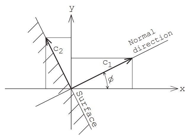
First, we calculate the velocity component $c_1$ perpendicular to the wall and the two parallel velocity components $c_2,c_3$. These can be calculated using the same equation as the generation of the velocity components of molecules flowing in from the boundary with a macroscopic velocity of zero.
$$\begin{array}{}\text{(60)}& c_1=\sqrt{-2R{T}_w{\log }_e{R}_{f1}}\end{array}$$ $$\begin{array}{}\text{(61)}& \theta =2\pi R_{f2}\end{array}$$ $$\begin{array}{}\text{(62)}& r=\sqrt{-2R{T}_w{\log }_e{R}_{f3}}\end{array}$$ $$\begin{array}{}\text{(63)}& c_2=r\sin \theta ,c_3=r\cos \theta \end{array}$$

Here, $T_w$ is the wall temperature.

Next, we convert these velocities to velocity components $u,v,w$ in the $x,y,z$ directions as follows:
$$\begin{array}{}\text{(64)}& u=c_1\cos \varphi -c_2\sin \varphi \end{array}$$ $$\begin{array}{}\text{(65)}& v=c_1\sin \varphi +c_2\cos \varphi \end{array}$$ $$\begin{array}{}\text{(66)}& w=c_3\end{array}$$

Another type of wall reflection is specular reflection. The angle of incidence and the angle of reflection are equal, and the molecular velocity does not change except for the reversal of the velocity component perpendicular to the wall, and there is no exchange of energy between the molecule and the wall. In general, such a surface does not exist, but this reflection occurs when a symmetrical surface is considered. There is also a method of simulating an intermediate reflection between the two by predetermining the ratio of diffuse reflection and specular reflection (accommodation coefficient). This method can be used in two ways: one is to determine whether each reflection is diffuse reflection or specular reflection using a random number, and the other is to combine the velocity component in each reflection from both diffuse reflection and specular reflection. The former is more common, but the latter method has the advantage that a lobular reflectance distribution can be easily achieved even with a single incident angle.

Ideally, the starting point of the reflected molecule should be a point on the wall, but in that case, calculation errors may cause the molecule to start from inside the wall, which can have a negative effect on the simulation. To prevent this, it is better to fly the molecule from a point slightly above the wall (a point a little into the flow field). How far the molecule should be above the wall depends on the shape of the wall, but about $1/1000\sim 1/100$ of the cell length is a safe bet. However, if the wall is concave, or if the wall equation is complex and errors are likely to occur in the calculation of the starting point, it is necessary to float it even more.

The routine for molecular movement starts from Line 239. After advancing the molecule number by one, the position coordinates and velocity components stored in the single precision array are temporarily replaced with double precision variables to reduce calculation errors. Now, for molecules that have been in the flow field from the beginning, the time step $\mathrm{\Delta }t$ is used as it is for the travel time, but for molecules that flow in from the boundary, a random multiple of $\mathrm{\Delta }t$ is given (lines 245-249). In other words, this is a treatment that takes into account that the molecule has already spent time before passing through the inflow boundary. If this is neglected, distortion will occur near the boundary. In line 250, the molecule is first moved unconditionally by $\mathrm{\Delta }t$. The IF block in lines 252-271 is the process that is performed when the $x$ coordinate of the molecule’s destination becomes negative. First, in lines 253-256, the time when the molecule reaches $x=0$ is calculated using equation (50), and the $y$ coordinate at that time is calculated using equation (57). If this $y$ coordinate is smaller than the orifice radius, the molecule will have flowed back through the orifice aperture, so in line 281, it is counted, and then the molecule is discarded from the calculation domain (lines 284-290). Also, if the $y$ coordinate is greater than the $y$-direction boundary EO of the flow field, it means that the molecule has flown out of the calculation domain before colliding with the orifice wall, so this is counted in line 283 and the molecule is discarded. Molecules that do not fall into either of the above two IF statements are reflected by the wall in lines 259-270. In lines 259 and 260, the molecular velocities $v,w$ just before colliding with the wall are calculated using equations (58) and (59), but these two lines are not directly required for this calculation. However, they are included in the program because they are required when calculating the balance of momentum and energy exchanged between the molecule and the wall, or when incorporating the characteristics of specular reflection as part of the reflection. After the time available for movement after reflection is calculated in line 261, the velocity components after reflection are calculated using equations (60)-(63) in lines 263-267. Since the normal vector of the orifice wall coincides with the $x$-axis, equations (64) to (66) are not necessary. Lines 268 and 269 determine the coordinates of the starting point of the molecule. As mentioned above, the $x$-coordinate is given by floating it above the orifice surface by $1/1000$ of the cell length. Then, line 270 determines the $x$-coordinate of the new destination.

Lines 272 to 279 process molecules that do not collide with the orifice wall or molecules that depart from the wall. In line 272, the outflow counter is advanced for molecules that have crossed the $x$-direction boundary ES of the flow field, and then the molecule discarding process is performed. For molecules that have not crossed the boundary, lines 273 to 275 calculate the $y$-coordinate after movement using equation (57). Using the $y$-coordinate, line 276 checks whether the $y$-direction boundary has been crossed. For molecules that have crossed the boundary, the outflow counter is also advanced and the molecule discarding process is performed. Molecules that do not fall under the above two IF statements will remain in the flow field, so after calculating the velocity components $v,w$ after movement using equations (58) and (59), in lines 293 to 297, the position coordinates and velocity component values ​​are converted from double-precision variables to single-precision arrays. In line 299, if the movement calculations for all molecules have not yet been completed, the process moves on to the movement of the next molecule.

Here, we will explain the molecule discarding process. Since the information of molecules that have jumped out of the calculation area is not needed, they will be discarded from the array that stores the information, but the molecular information is stored randomly in the array. Therefore, simply discarding them will leave the array in a worm-eaten state. In other words, in order to store the information of new molecules that will flow in, it is necessary to organize the array. Therefore, as shown in lines 284 to 290, the information stored at the end of the array at that time is transferred to the element that stored the molecular information to be discarded, and the number at the end of the array (total number of molecules) is decremented by one.

In lines 300 to 303, after all the calculations for the movement of the molecules that were in the flow field from the beginning are completed, the process moves on to the process of starting the calculation of the movement of the molecules flowing in from the boundary. Once that calculation is also completed, check the update of the maximum number of molecules, and then move on to the routine of “calculation to determine which cell the molecule is in”.

<Assignment> Draw a flow chart for the “spatial movement routine of molecules” in the example program and track the movement of the molecules.

15. Calculating the cell to which the molecule belongs and sorting the molecules on the cross-reference array

Before proceeding with the calculation of intermolecular collisions, a procedure is required as a preparation. Since the position coordinates change due to the spatial movement of the molecules, first survey which cell each molecule belongs to. In the example, in lines 392 to 394, the sequence number in the $x$ direction of the cell to which the molecule belongs is calculated using equation (13). However, 0.999999 is used instead of 1 in equation (13) to induce the value to be lower and convert it to an integer, and if the cell number becomes zero, it is changed to 1. This is an operation to prevent calculation errors.

On the other hand, in the $y$ direction, the cell sequence numbers are first calculated by simple division as equally divided cells, as mentioned above. The three cells closest to the central axis are combined into one, and this processing also have the calculation error countermeasures (lines 396-401). In line 403, the cell sequence numbers in both the $x$ and $y$ directions are used to determine the cell numbers assigned consecutively throughout the entire region. It is a good idea to check for stray molecules (error molecules) during this calculation process. That is, there is a small probability that a molecule may enter within the wall due to a calculation error, or a molecule that should have jumped out of the calculation region may still survive for some reason. If these molecules are left as they are, they may cause a fatal error in the entire simulation. Therefore, these molecules are checked at this point, the number of error molecules is counted, and appropriate processing is performed at the same time. Lines 383-390 and 404-407 correspond to this. In addition, by constantly monitoring the error counter (outputting it to the monitor), we can also check for program bugs (if the number of errors is abnormally high, it is possible that there is an error in the program). In the example, this is done in line 227.

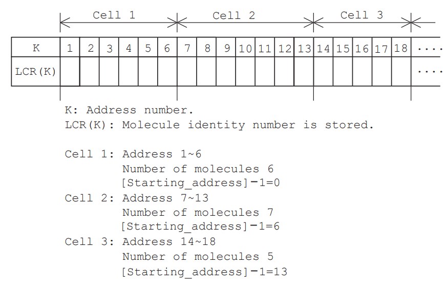
Now, to make it easier to calculate intermolecular collisions, we need to process the rearrangement of the molecules in the cross-reference array LCR(K) in the order of the cells to which they belong. Figure 4 shows an example of the array created by this process, where K represents the seat number (address), and the molecule number (molecule identification number) is stored in LCR(K). In Figure 4, the first cell has 6 molecules, reserves 6 seats from 1 to 6, and the seat number just before the first seat (starting_address$-1$) is 0. Similarly, the second cell has 7 molecules, reserves 7 seats from 7 to 13, and the seat just before the first seat is 6. The third cell has 5 molecules, reserves seats from 14 to 18, and the seat just before the first seat is 13.

To create this cross-reference array, first, the number of molecules in the cell is investigated for all cells. That is, in lines 414 to 418, the number of molecules in the cell, IC1(N), is set to zero, and then the number of molecules in the cell is counted while checking the cells to which all molecules belong. Next, in lines 419 to 423, the number of molecules in the cell is accumulated in the order of cells, and the first seat of each cell on the LCR(K) array is investigated. In fact, the seat number just before the first seat of each cell, starting_address$-1$, is stored in IC2(N). At that time, the number of molecules in the cell, IC1(N), is cleared to zero again. Finally, in lines 424 to 428, the number of molecules in the cell to which each molecule belongs is counted, and the molecule numbers are filled in the seats on the cross-reference array in order using IC2(N). Now, as an example of using this cross-reference array, let us consider the case where a molecule is arbitrarily selected from the target cell in the first stage of an intermolecular collision. If we randomly select one of the consecutive seat numbers given to the cells, we can use this array to cross-reference the molecule number, and as a result, we can obtain the velocity components of the molecules involved in the collision.

16. Program for intermolecular collisions – collision calculation part 3

The calculation of intermolecular collisions is performed for each cell in a DO loop (lines 433 to 509) that spans all cells. In line 435, if there are not two or more molecules in a cell, the collision calculation for that cell is skipped. Lines 436 and 437 calculate the number of trials (number of collision attempts) for selecting a colliding molecule pair using equation (34). As mentioned earlier, the collision cross section ${\sigma }_T$ needs to be increased by the amount that the number of simulated molecules is smaller than the number of real molecules, so this is corrected using the weighting factor WEI. Lines 438 to 440 are operations that convert the real number of collisions into integers using random numbers. The collision pair check is repeated the number of collision trials ICN obtained in this way, and if a collision is possible, an actual calculation of an intermolecular collision is also performed (lines 442 to 507).

Lines 444 to 447 are the calculation to randomly select one of the molecules in the cell using the number of molecules in the cell IC1(N), the starting_address$-1$ (the first seat number$-1$) IC2(N), and the cross-reference array LCR(K). Here, the seat number is lowered by adding 0.9999999 and truncating the decimal point, and if the number is too small, 1 is added. This operation is a countermeasure against calculation errors, as explained before. Line 447 converts the seat number to a molecule number using the cross-reference array. Similarly, lines 449 to 453 are a calculation to select another molecule. However, a process is added to avoid selecting the same molecule. Lines 455 to 459 calculate the relative velocity of the two molecules. RVRALL and RVRGT in lines 461 and 462 are variables that check whether the estimate of $({\sigma }_T{c}_r{)}_{max}$ is valid. If RVRGT is sufficiently smaller than RVRALL, there is no problem. Lines 226 and 227 output the progress of this ratio OV. Line 463 calculates the collision probability of the molecular pair using equation (35). However, the parts common to the numerator and denominator of equation (35) are omitted. In line 465, if the uniform random number is smaller than the collision probability, this molecular pair will collide, and lines 467 and onwards are executed, but if it is greater than the collision probability, the collision trial for the next pair will proceed.

Lines 468-473 calculate the relative velocity components of VHS molecules after collision using equations (20)-(24), and lines 475-492 calculate the relative velocity components of VSS molecules after collision using equations (26), (28)-(32). Line 495 counts the number of collisions and is not used directly in this example. Lines 497-505 calculate the velocity components of both molecules after collision using equations (36)-(38). Here, VCCM is the center of mass velocity, but since the molecules have the same mass, $m_1$ and $m_2$ do not appear in the program.

17. Sampling of flow field data

The above-mentioned molecular movement and intermolecular collisions are repeated endlessly to form a flow field, but the only things that change in the computer are the position coordinates and velocity components of the many molecules. The information we actually want from the flow field is density (number density), flow velocity, and temperature, so we need to calculate them. The number density can be calculated from the number of molecules in each cell, $N$

$$\begin{array}{}\text{(67)}& N=\sum _{i=1}^{N}1\end{array}$$ and the cell volume, $V_{cell}$. The flow velocities, $U$, $V$ and $W$, can be obtained by averaging the velocities of the molecules in the cell.

$$\begin{array}{}\text{(68)}& U=\frac{1}{N}\sum _{i=1}^N{u}_i,V=\frac{1}{N}\sum _{i=1}^N{v}_i,W=\frac{1}{N}\sum _{i=1}^N{w}_i\end{array}$$ In the case of monoatomic molecules, the temperature, $T$, can be calculated by subtracting the “kinetic energy due to the flow velocity” from the “translational energy of the gas molecules” (in the case of polyatomic molecules, the rotational and vibrational energy of the molecules is also taken into account). For example, the temperature in the x direction, $T_x$, is as follows:

$$\begin{array}{}\text{(69)}& T_x=\{\frac{1}{N}\sum _{i=1}^N{u}_i^2-(\frac{1}{N}\sum _{i=1}^N{u}_i{)}^2\}/R\end{array}$$The same procedure is used for $T_y$ and $T_z$, and the temperature, $T$, is calculated as the average of these.

$$\begin{array}{}\text{(70)}& T=(T_x+T_y+T_z)/3\end{array}$$

When calculating pressure, if the equation of state holds, it is calculated from the density and temperature. If the equation of state cannot be used due to a strong non-equilibrium condition, a virtual wall is placed at the position where the pressure is to be calculated (in the program) and the pressure is calculated from the momentum of the molecules passing through it.

In the example, the DO loop starting from line 514 is a sampling process for the information in the cell. For each molecule, the cell to which it belongs is investigated, and in line 517 the number of molecules is counted using equation (67), in lines 518 to 520 $\sum u_i$, $\sum v_i$, and $\sum w_i$ in equation (68), in line 521 $\sum u_i^2$ in equation (69), and in lines 522 and 523 $\sum v_i^2$ and $\sum w_i^2$. The final density, velocity, and temperature values ​​are calculated in the data processing routine at the end of the program.

Intermediate summaries of the in-cell sampling data are output to a file every K100 times.
Lines 529 and 530 determine whether the number of times for data output has been reached. If the number of times has been reached, lines 531 to 591 are executed, and if the number of times has not been reached yet, the program returns to line 224.
The file name output every K100 times is different each time. That is, they are named ‘sjetc01’, ‘sjetc02’, …. Lines 531-542 determine the name, and lines 544-553 output the cell information to a file.

The other output file is the net number of passing molecules at the orifice inlet and downstream boundary. In this example, it is non-dimensionalized by the number of incident molecules at the stagnation point $(1/4)n\bar{c}$, and this is done in lines 556-561. ‘A‘ in line 556 is a coefficient to express the number of passing molecules as the number of real molecules, but it has no meaning in this example. Note that this non-dimensional number of passing molecules becomes the non-dimensional conductance if the downstream pressure (pressure ratio 1/50 in this case) is ignored. This output file is always output with the same file name ‘sjet4’, but it is set to output both the “individual data output up to that point” and the “average value from the latest data back to those individual data”. The example problem calculates the steady state of a free jet, but with the DSMC method, the flow always experiences an unsteady state before reaching a steady state. Therefore, it is necessary to estimate at which point in the output data the flow reached steady state, and this can be done using the data on the number of passing molecules. In other words, if the average value calculated going back from the most recent data is stable, then it can be said that the flow has almost reached steady state. To be more precise, it is better to use a statistical calculation using a $t$ distribution table, taking into account the error range from the average value. Lines 563 to 584 perform the averaging operation and then output the file. Lines 586 to 591 initialize (zeroing) the array variables SS and SC.

18. Final Data Processing

In the example program, the final data processing routine is created separately from the main routine. In other words, once the simulation is finished, the number of output data to average is determined as described above, and the program is executed again. Entering ‘2’ in lines 205 to 207 will move to the data processing routine. XLIM in line 601 inputs how many times the orifice diameter the flow field length should be processed in the $x$ direction. Since the downstream boundary in the example has a boundary condition of an infinitely far downstream state, there is a possibility that the results will be distorted, especially near the downstream vertical boundary perpendicular to the central axis. Therefore, in order to truncate the data near the boundary, for example, in this calculation, enter a value of about ’10’ to be more generous (enter ’16’ if you want to know the degree of distortion). The following input data KDO1 and KDO2 are the start and end numbers of the processing data. In this calculation, we think that the steady state may be reached after the sixth iteration, so we enter ‘6’ and ’20’. Of course, we can also observe the unsteady state by entering the same number, for example ‘1’, for both the start and end numbers. However, since this is an unsteady result averaged over a fairly long time, it is not an unsteady state in the strict sense. Lines 607 to 634 read cell information from multiple files and perform averaging.

Lines 636 to 671 are the routines that calculate the final flow field data and output it to the file ‘OUTD’. The control variable I in DO 302 changes in the order of the cells arranged in the $y$ direction, and the control variable J in DO 303 changes in the order of the cells arranged in the $x$ direction. Lines 639 to 643 calculate the $y$ coordinate of the cell center. The three cells closest to the central axis are connected, so the above calculation is performed. Lines 646 to 648 calculate the $x$ coordinate of the cell center. Lines 649 and 650 normalize the cell center coordinates with the orifice diameter, and line 651 is the process when the $x$ coordinate exceeds the data processing cutoff point. Lines 652 to 654 express the density of each cell with the stagnation point density set to 1 (non-dimensionalization by stagnation point density). Lines 655 to 657 calculate the flow velocity using equation (68), and lines 658 to 660 calculate the temperature in each direction using equation (69). Line 661 calculates the average temperature using equation (70), and line 662 is the average temperature perpendicular to the central axis. Lines 663 and 664 calculate the Mach number by dividing the flow velocity by the speed of sound $\sqrt{\gamma RT}$ ($\gamma$ is the specific heat ratio). When outputting to a file on lines 665 and 666, the velocity is made dimensionless by the most probable molecular thermal speed at the stagnation point $c_{max}^{\prime }$, and the temperature is made dimensionless by the stagnation point temperature.

The output data is arranged in the following order for each cell: $x$ coordinate, $y$ coordinate, density, velocity in the $x$ direction, velocity in the $y$ direction, average temperature, temperature parallel to the axis, temperature perpendicular to the axis, and Mach number. The data is arranged as parametric data, so that three-dimensional graphs (bird’s-eye views) can be directly drawn using the free software ‘gnuplot’.

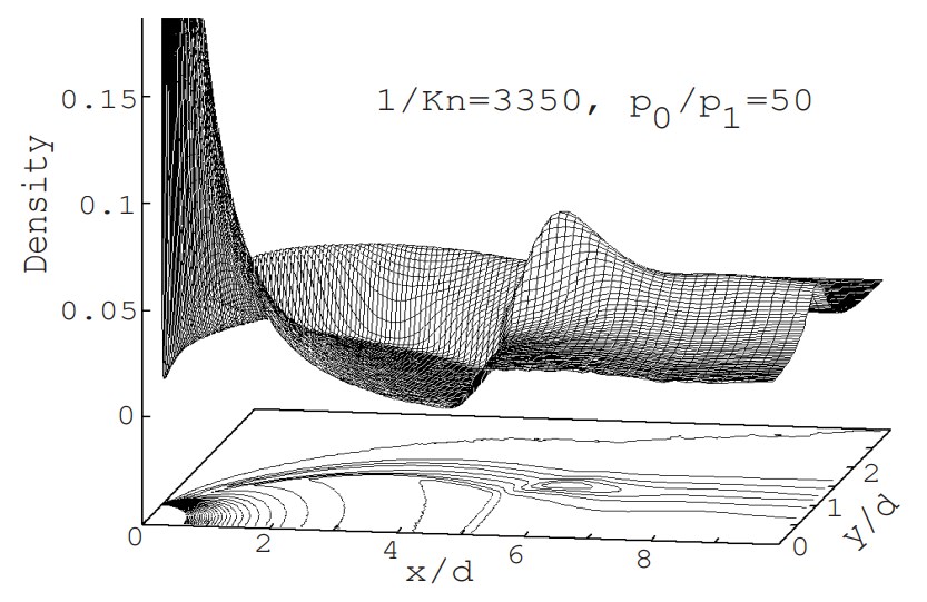
Figure 5 shows the density distribution calculated in the example, processed by gnuplot (v3.5). It is expanded in the height direction, so the Mach disk and barrel shock can be clearly observed. However, in the example, the calculation area is not set upstream of the orifice, so the flow rate is larger than it actually is, and the jet itself is larger, and the Mach disk is shifted downstream from its original position.

<Assignment> When considering the effect of back pressure on jet formation, depending on the flow field conditions, the effect of the downstream peripheral boundary parallel to the jet axis may be dominant, and the downstream vertical boundary perpendicular to the jet axis may have almost no effect. In the example program, perform a calculation by setting only the downstream vertical boundary as a complete vacuum, and compare the results.

19. Development from the example program

The trick to making a good program is to create many programs yourself. We hope that you will use this example program as a basis to challenge yourself to more complex problems. Finally, some development tasks are added.

[1] In the example, the free jet is large because there is no computational domain upstream of the orifice, and the shape of the jet immediately after the orifice exit is slightly different from the actual shape. Therefore, create a program with a computational domain upstream and perform a DSMC calculation. In that case, how should the boundary conditions at the upstream boundary be set?

[2] Give the orifice a thickness. Also, how can you make it a conical nozzle?

[3] In the example, the cell length is changed depending on the location. If the time step could also be changed depending on the location, efficient calculations would be possible in situations with a large pressure ratio. How can this be achieved? (Difficult problem)

[4] The example shows an axisymmetric flow field, but if the flow field could be made three-dimensional, a free jet passing through a rectangular orifice could also be calculated. How should the example program be modified?

[5] What part of the example program should be modified to realize a mixed gas flow?

To see the example program, please click here. (Please note that the one to three digits and the space following them on the left side of each line in the program indicate the line number (1 to 677) and are not included in the program itself.)