(The description in English is shown after the Japanese sentence.)
(以下は,最初の記述を2022年5月に行いましたが,その後,修正を行っています.)
本ブログを作成・運営する Masa です.定年退職した老人ですので,とりあえず約3年かけて,ゆっくりと一通りを完成させていくつもりです.一番の目的は,家庭であまり使われずに遊んでいるノートPCあるいはデスクトップPCを用いて,皆さんに,DSMC法(Direct simulation Monte Carlo method)[文献 1),2),3)] による流れのシミュレーションを体験して頂こうというものです.PC の OS は 64ビットWindows が必要.CPUは intel か AMD.Core や thread の数は多いほど並列処理で速くなるが,シングルCoreでも時間をかければできる (計算時間の例として,「2. 試し計算」内の「8. 複数のPCでの JET-P3S1 の計算時間比較」を参照).なお,複数のCPUチップを持つPCの場合,本ブログでは,異なるCPUチップの core や thread を結びつけて並列計算することはできません.現在考えている予定は,次のとおりですが,今後変更するかも知れません.
(1) DSMC法の概要とU_systemの解説を記述
(2) Jet(超音速噴流)を中心とした計算ソフトの公開・配布(計算実行のための.EXEファイルと入力データ例の提示が主ですが,興味をお持ちの方のために,一部,Fortranソース基礎コードとU_systemコードも入れる予定です).
(3) これまでの私の計算例を表示
(4) 2024年と2026年に,DSMC法による乱流解析の項目も加えました.
なお,下記のものが必要になるかも知れないので,あらかじめインターネットを通じてご用意して頂くとよいと考えます.いずれも無料でダウンロードできます(ダウンロードに至る操作の途中で,大きなダウンロードボタンによって有料サイトに誘われることがあるので注意してください).
(1) 計算結果を表示するためのツール gnuplot (私が持つバージョンは v5.4).なお,tecplot(このソフトは有料で高価)を利用できる方は,gnuplot は必要ありません.
(2) .avi ファイルの表示を可能にするためのコーデック K-Lite Codec Pack(ただし必要ないかも知れない).
(3) 圧縮ファイルを解凍するためのツール(例えば,7-zip.ただし必要ないかも知れない).
——————–お詫び——————–
下記アニメーションに関し,圧力比4の中に圧力比2の結果が紛れ込んでいましたが,2024年6月の時点で修正を行いました.
——————–Apologies——————–
Regarding the animation below, the results for a pressure ratio of 2 were mixed in with the results for a pressure ratio of 4, but this was corrected as of June 2024.
<計算結果の一例> Examples of calculations
下記の例に関する詳しい説明は,第4章を参照してください.第4章の計算結果.
For detailed explanations of the examples below, please see Chapter 4. Calculation results for Chapter 4.
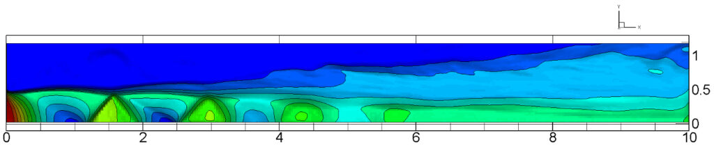
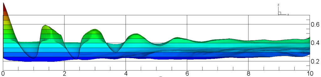
Result animation: Disturbance of supersonic jet boundary
(density distribution, upstream pressure 1 atm, pressure ratio 4)
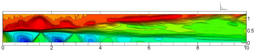
Result animation: Disturbance of supersonic jet boundary
(temperature distribution, upstream pressure 1 atm, pressure ratio 4)
密度分布も温度分布も,共に,上段は,渦の定常振動形成後に約42μ秒間平均して作成した結果(人間の目視に比較的近い).下段は,噴流の流れ始めから渦の定常振動が形成されるまでを,各画面約1μ秒の平均で作成して繋ぎ合わせた結果(高速度撮影によるスローモーション再生に該当).
In both density distribution and temperature distribution, the upper part of the examples of calculations is the result of averaging about 42 μs after the formation of the steady vibration of the vortex (relatively close to human visual observation). The lower part is the result of creating and stitching together the images from the beginning of the jet flow to the formation of the steady vibration of the vortex, with an average of about 1 μs for each screen (corresponding to slow motion playback by high-speed photography).
(先頭表紙に戻る: Return to the top cover page)
1. Greetings
(The following text was originally written in May 2022 but has since been revised.)
This is Masa who creates and manages this blog. I’m an old man who retired, so I’m going to slowly complete the whole process over three years. The main purpose is to let everyone experience the flow simulation by the DSMC method (Direct simulation Monte Carlo method) [Reference 1),2),3)] using a notebook (laptop) PC or desktop PC that is rarely used at home. The OS of the PC requires 64-bit Windows. The CPU is Intel or AMD. The larger the number of Cores and threads, the faster the parallel processing, but even a single Core can be done if it takes time (See “8. Some examples of calculation time for ‘JET-P3S1’ by various PCs with multi-core or multi-thread processor” in “2. Test Calculation“). In the case of a PC with multiple CPU chips, in this blog, it is not possible to connect cores and threads of different CPU chips for parallel calculation.
The current plan is as follows, though it may be subject to change:
(1) Provide an overview of the DSMC method and an explanation of U_system.
(2) Release and distribute simulation software focused on supersonic jets (primarily consisting of executable [.EXE] files and sample input data; however, for those interested, I also plan to include some basic Fortran source code and U_system code).
(3) Present examples of simulations I have conducted to date.
(4) Include topics on turbulence analysis using the DSMC method (added in 2024 and 2026).
The following items may be required, so it is recommended that you prepare them in advance via the Internet. Both can be downloaded for free (please be careful not to be led a pay site by a large download button during the operation leading up to the download).
(1) Tool for displaying calculation results gnuplot (my version is v5.4). If you can use tecplot (this software is charged and expensive), you do not need gnuplot.
(2) K-Lite Codec Pack (although it may not be necessary) to enable display of .avi files.
(3) A tool for decompressing compressed files (for example, 7-zip. it may not be needed).
<Examples of calculations>
For detailed explanations of the examples below, please see Chapter 4. Calculation results for Chapter 4.
(density distribution, upstream pressure 1 atm, pressure ratio 4)
(temperature distribution, upstream pressure 1 atm, pressure ratio 4)
In both density distribution and temperature distribution, the upper part of the examples of calculations is the result of averaging about 42 μs after the formation of the steady vibration of the vortex (relatively close to human visual observation). The lower part is the result of creating and stitching together the images from the beginning of the jet flow to the formation of the steady vibration of the vortex, with an average of about 1 μs for each screen (corresponding to slow motion playback by high-speed photography).