(日本語による解説はここをクリック）

One of the features of the DSMC method is that it divides the physical space into minute spatial elements called cells, and calculates intermolecular collisions between molecules that exist in the same cell. For this reason, the cells must be very small, and ideally, one side of the cell must be less than the mean free path (some reports have said that less than 1/3 of the mean free path is necessary depending on the calculation target). This condition would not be a big problem in outer space, where the density is very low, but if it is atmospheric pressure, for example, the mean free path is about 0.066 μm, and 15,000 cells are required for a length of 1 mm, and 2.3 × 10${}^8$ cells for an area of ​​1 mm${}^2$. The number of molecules required is several times that amount, so it cannot be handled by a small PC and the calculation time will be enormous. Of course, even if the cells are larger than the mean free path, the results will not be completely useless, but it is inevitable that they will lack precision.

When I was explaining the distribution function of the equilibrium molecular velocity (Maxwell distribution) in my university lectures, I wondered if we could make the cell larger by making good use of this Maxwell distribution, which was the trigger for devising this U_system. In normal intermolecular collisions in the DSMC method, molecules in the same cell are all calculated as being in the same position (for example, the center of the cell) even though they are in different positions within the cell. The larger the cell is beyond the mean free path, the more molecules that are far away in the cell and should not collide are calculated as colliding, creating distortions in the results. So, what if, when two molecules collide, we add corrections to the molecular velocity components according to their original positions? In that case, can we use the equilibrium distribution function? This is the underlying idea of ​​the U_system.

In the following, we will use an example program for the U_system to explain the U_system, and this is the basic program for the DSMC method explained in Section 5.1 with the U_system part added. Therefore, you should have a good understanding of Section 5.1 and the basic programs that accompany it. In the explanation of U_system, we use notations such as “see line XX to line XX” in the example program, but rather than a detailed explanation like in section 5.1, we keep it to a rough explanation, and the variable symbols in the explanation do not necessarily match the variable symbols in the Fortran program, so please read it with great care. Regarding the U_system code, in addition to the supersonic jet in the axisymmetric flow field used here, the code for one-dimensional normal shock waves is also included in the electronic appendix of Reference(9), so please refer to that as well.

As mentioned earlier, in conventional collision calculation methods, as the cell becomes larger, the positions of the two colliding molecules become proportionally farther apart, so the simulation is not performed faithfully. Ideally, two colliding molecules should be selected at the same position, but in a simulation that uses only a finite number of molecules, it is difficult to find two molecules in the exact same position even if the cell is made smaller.

In U_system, the molecular velocity is corrected just before the collision calculation as if one molecule P was aligned with the position of the other molecule Q. Now, we assume that all molecules in the flow field follow the velocity distribution function of a local equilibrium state with a certain temperature and flow velocity (Maxwell distribution or Maxwellian). In the following, the correction formula is derived assuming that the velocity distribution function at the two molecular positions is a Maxwell distribution, but the obtained correction formula itself is valid even if the distribution function at the two positions is not necessarily a Maxwell distribution (for example, the exponential function that appears in the Maxwell distribution formula can be replaced with another function). The only necessary condition is that “the distribution shape is such that the center of distribution moves in parallel to the left and right according to the flow velocity, and the peculiar or thermal velocity component of the molecules is proportional to the square root of the temperature.” Because two molecules are in the same cell even large cell, it is not particularly difficult to satisfy the above conditions, even if the distribution is not Maxwellian.

Now, let us assume that the distribution function of the position of molecule P is $f_1$, the distribution function of the position of molecule Q is $f_2$, and the velocity of molecule P is at point A on $f_1$ (Fig. 1).

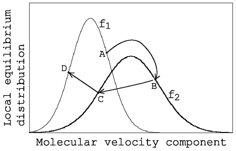
When calculating collisions, this point A should be moved somewhere on the distribution function $f_2$ , and the method I thought was the most natural is to move it so that the position of point A on $f_1$ and the position on $f_2$ are relatively the same (point B). The calculation to find the position of point B is simple. Now, considering the distribution function of the $x$-direction velocity component $u$, $f_1$ and $f_2$ can be written as the following equations (1) and (2). Here, $R$ is the gas constant, $T_{x1}$ and $T_{x2}$ are the temperatures defined by the $x$-direction velocity component of the three temperature components based on the translational motion of molecules (hereinafter referred to as $x$-direction temperatures), and $U_1$ and $U_2$ are the $x$ components of the flow velocity.
$$\begin{array}{}\text{(1)}& f_1=\frac{1}{\sqrt{2\pi R{T}_{x1}}}\exp \{-\frac{(u_A-U_1{)}^2}{2R{T}_{x1}}\}\end{array}$$

$$\begin{array}{}\text{(2)}& f_2=\frac{1}{\sqrt{2\pi R{T}_{x2}}}\exp \{-\frac{(u_B-U_2{)}^2}{2R{T}_{x2}}\}\end{array}$$

If $f_1$ and $f_2$ are made dimensionless at their maximum values ​​and are set equal, the following equation is obtained.

$$\begin{array}{}\text{(3)}& \frac{(u_A-U_1{)}^2}{T_{x1}}=\frac{(u_B-U_2{)}^2}{T_{x2}}\end{array}$$

Therefore, the following equation is obtained.

$$\begin{array}{}\text{(4)}& u_B=U_2+(u_A-U_1)\sqrt{\frac{T_{x2}}{T_{x1}}}\end{array}$$

Using this corrected velocity $u_B$ (note that $u_A$ is the velocity before correction), subsequent calculations are performed using the general collision calculation method (Bird’s method). The resulting post-collision velocity $u_C$ (point C) is corrected again using the following equation as molecule P returns to its original position (point D).

$$\begin{array}{}\text{(5)}& u_D=U_1+(u_C-U_2)\sqrt{\frac{T_{x1}}{T_{x2}}}\end{array}$$

$v$ and $w$ are also corrected in the same way, but in two-dimensional problems (axisymmetric problems), only $T_x$ and $T_{yz}$ are used for the temperatures (there is also a method of using $T_y$ and $T_z$ instead of $T_{yz}$), and $W$ is not used to correct the flow velocity $w$. In one-dimensional problems, temperatures $T_x$ and $T_{yz}$ are used, but $V$ and $W$ are not used to correct the flow velocities $v$ and $w$. Although it is called U_system, as shown above, one molecule of a collision pair appears to move to the position of the molecule that it collides with and then returns to its original position after the collision, so U is used to mean a U-turn, and the whole mechanism that performs this operation for all collision pairs is called system, and so it is named this way. If there is no change in the flow velocity and temperature within the cell, it will be the same as a general collision calculation method.

Here, to use equations (4) and (5), data on the flow velocity $U$ and temperature $T$ at the positions of molecules P and Q is required. Assuming that the data at the edges of the cell is known, simple linear interpolation is used for one-dimensional problems, bilinear interpolation for two-dimensional problems, and trilinear interpolation for three-dimensional problems. The data at the edges of the cell is derived from the values ​​at the centers of adjacent cells. The example program is an axisymmetric problem, and bilinear interpolation is used using the values ​​at the four corners of the cell, so the formula for this is shown below.

<Bilinear Interpolation> How to find the flow velocity and temperature at any position within a cell in a two-dimensional problem (axisymmetric problem):

If the coordinates of the four corners of a rectangular cell are ($x$, $y$), ($x+A$, $y$), ($x$, $y+B$), ($x+A$, $y+B$), and the temperatures at these points are $T_1$, $T_2$, $T_3$, $T_4$, then the temperature at any position ($x+a$, $y+b$) within the cell can be found by

$$\begin{array}{}\text{(6)}& T=(1－b/B)\{(1－a/A)T_1+(a/A)T_2\}+(b/B)\{(1－a/A)T_3+(a/A)T_4\}\end{array}$$

The same is true for the flow velocity. By the way, there is a simple way to experience this bilinear interpolation, although it is not exact. There is a cooking tool called a “makissu (rolling mat)” that is used to make sushi rolls in Japanese cuisine, and it can be purchased for 110 yen at large 100-yen shops. First, stretch it taut with both hands to create a square plane, and then twist both hands in an appropriate way to create any smooth curved surface. Makissu are made by weaving straight bamboo strips with string, so they are basically linear, but it is possible to obtain a smooth curved surface. The formula for trilinear interpolation using the data of the eight corners of a cell when applied to a three-dimensional problem is a little complicated, but it is recommended that readers derive it as an exercise.

Now, for the first calculation only, the flow velocity and temperature of each cell are obtained using the conventional DSMC method (Bird method). In the long iterations of the DSMC method, the calculation using the conventional method is only required the first time, and thereafter, the flow velocity and temperature data are updated sequentially by U_system. Although the time required for one calculation with the U_system is longer than with conventional calculation methods, considering that the cells can be made larger, the U_system has an advantage in terms of time comparison for the entire calculation.

However, when correcting for molecular velocity, the momentum and energy of each colliding molecular pair are not strictly conserved before and after the collision. Of course, if the average is taken for the entire flow field or over a long period of time, they will be conserved within the range of statistical variation. However, after examining many calculation examples, it was found that if there is a large difference in energy before and after a collision in a single collision, this can cause distortion in the results to grow, especially in a flow field with rapid changes such as shock waves occurring in the range of several cells. Therefore, improvements were made to conserve energy before and after the collision, and the calculation stability of the U_system was greatly improved (U_system-3). However, it was pointed out that the conservation of momentum was not guaranteed, and there were also cases where temperature increases unexpectedly occurred depending on the calculation conditions, so further improvement was desired. Sun et al. (Reference 7) considered that intermolecular collisions take place in a dimensionless velocity space, and performed DSMC analysis by introducing the concept of using flow velocity and temperature as scale variables to make the velocity dimensionless (LCDSMC method). The calculation method is basically the same as the U_system that I proposed, but what is noteworthy is that the correction method proposed by Pareschi et al. (Reference 8) was adopted to strictly conserve the momentum and translational energy of the molecules for each cell. The method is explained next.

When the velocities of many molecules are reproduced using random numbers from the velocity distribution function of a local equilibrium state with a given flow velocity and temperature, even if the flow velocity and temperature are calculated in reverse from the reproduced molecular velocities, they do not strictly return to the original state. To strictly return to the original state, Pareschi et al. devised a method for strictly conserving momentum and energy. Now, let us consider applying this method to the U_system. Let the molecular velocity components before and after the collision be $u$, $v$, $w$ and $u^{\ast }$, $v^{\ast }$, $w^{\ast }$, and finally become $u^{+}$, $v^{+}$, $w^{+}$ by strictly conserving momentum and energy using the correction method of Pareschi et al. In this case, the correction is performed using four parameters ${\lambda }_X$, ${\lambda }_Y$, ${\lambda }_Z$, $\tau$ as shown in equation (7). (Note) The same symbol $\tau$ as used for the mean free time in section 5.1 is used, but this is in accordance with the original paper by Pareschi et al., so please be careful not to confuse them. Note that the variable symbols in the Fortran program are TAU for the mean free time and ATAU for the correction parameter.
$$\begin{array}{}\text{(7)}& u^{+}=(u^{\ast }-{\lambda }_X)/\tau , v^{+}=(v^{\ast }-{\lambda }_Y)/\tau , w^{+}=(w^{\ast }-{\lambda }_Z)/\tau \end{array}$$

Here, to find ${\lambda }_X$, ${\lambda }_Y$, ${\lambda }_Z$, $\tau$, we use the momentum conservation equation and energy conservation equation shown in the following equations (8) to (11). Note that $m$ is the molecular mass, and the subscript $i$ means that the sum is to be found for all molecules.

$$\begin{array}{}\text{(8)}& \sum m_i(u_i^{\ast }–{\lambda }_X)/\tau =\sum m_i{u}_i\end{array}$$

$$\begin{array}{}\text{(9)}& \sum m_i(v_i^{\ast }–{\lambda }_Y)/\tau =\sum m_i{v}_i\end{array}$$

$$\begin{array}{}\text{(10)}& \sum m_i(w_i^{\ast }–{\lambda }_Z)/\tau =\sum m_i{w}_i\end{array}$$

$$\begin{array}{}\text{(11)}& \sum m_i[\{(u_i^{\ast }-{\lambda }_X)/\tau {\}}^2+\{(v_i^{\ast }-{\lambda }_Y)/\tau {\}}^2+\{(w_i^{\ast }-{\lambda }_Z)/\tau {\}}^2]=\sum m_i(u_i^2+v_i^2+w_i^2)\end{array}$$

As a result, $\tau$, ${\lambda }_X$, ${\lambda }_Y$, ${\lambda }_Z$ can be calculated using the following series of equations.

$$\begin{array}{}\text{(12)}& \tau =\pm \sqrt{[\sum m_i\sum \{m_i(u_i^{\ast 2}+v_i^{\ast 2}+w_i^{\ast 2})\}–A^{\ast }]/[\sum m_i\sum \{m_i(u_i^2+v_i^2+w_i^2)\}–A]}\end{array}$$
$$\begin{array}{}\text{(13)}& A^{\ast }=(\sum m_i{u}_i^{\ast }{)}^2+(\sum m_i{v}_i^{\ast }{)}^2+(\sum m_i{w}_i^{\ast }{)}^2\end{array}$$ $$\begin{array}{}\text{(14)}& A=(\sum m_i{u}_i{)}^2+(\sum m_i{v}_i{)}^2+(\sum m_i{w}_i{)}^2\end{array}$$

　

$$\begin{array}{}\text{(15)}& {\lambda }_X=(\sum m_i{u}_i^{\ast }–\tau \sum m_i{u}_i)/\sum m_i\end{array}$$

$$\begin{array}{}\text{(16)}& {\lambda }_Y=(\sum m_i{v}_i^{\ast }–\tau \sum m_i{v}_i)/\sum m_i\end{array}$$

$$\begin{array}{}\text{(17)}& {\lambda }_Z=(\sum m_i{w}_i^{\ast }–\tau \sum m_i{w}_i)/\sum m_i\end{array}$$

The U_system included in this blog strictly conserves momentum and energy as shown above. When calculating τ, it is necessary to use a positive sign before the square root. The conservation law is satisfied even if it is negative, but if it is negative, the correction parameters ${\lambda }_X$, ${\lambda }_Y$, ${\lambda }_Z$ will become very large values ​​in order to match the velocity direction before and after correction (the correction values ${\lambda }_X$, ${\lambda }_Y$, ${\lambda }_Z$​​ and the absolute value of the flow velocity will be almost the same magnitude). On the other hand, if it is positive, ${\lambda }_X$, ${\lambda }_Y$, ${\lambda }_Z$ are less than 1/100 of the flow velocity. Since equation (7) is originally used for correction and it is assumed that the difference before and after correction is small, the smaller difference will be used. Even in the results of actual application, if a negative sign is used before the square root, the conservation law is satisfied, but the effect of the U_system is almost lost. Incidentally, it is thought that if Pareschi et al.’s strict preservation method is applied to the Nambu method (modified Nambu method) (Reference 20), it may be possible to compensate for the shortcomings of the Nambu method.

The Fortran program USYS2024-3NEG.F (click here to jump to the program) is the original basic program in section 5.1 with the U_system part added (or modified), and the lines after the line ‘C2024-11-1 CUxx’ are the added parts. Note that the ‘xx’ after CU is numbered 1 to 9, and there are a total of nine places. The first line of each has ‘xx-start’ at the end, the last line has ‘xx^end’ at the end, and there is an additional part in between. Specifically, CU1 is 2 lines, CU2 is 8 lines, CU3 is 16 lines, CU4 is 14 lines, CU5 is 4 lines, CU6 is 1 line, CU7 is 249 lines from lines 573 to 821, CU8 is 112 lines from lines 872 to 983, and CU9 is 15 lines. The last CU9 part has ‘C’ at the beginning of every line, so it is a comment line and does not function, but if you remove this ‘C’, a plot file for tecplot will be created (if left as is, it will be a plot file for gnuplot).

The CU1 part changes the array of the original program from memory saving 4-byte single precision real numbers to 8-byte double precision real numbers, and this change was made to accurately check whether the conservation of energy and momentum is being performed correctly in the intermolecular collision process of U_system.

Before explaining the CU2 part, please remember that the cells of the space are arranged in a regular lattice on a two-dimensional plane. In present the grid size is 164×240, but in case we need to use the area upstream of the orifice in the future, KST9=260, KOT9=240 in the PARAMETER statement on line 51. Cells with the same $x$ coordinate have the same width even if the $y$ coordinate is different, and cells with the same $y$ coordinate have the same height even if the $x$ coordinate is different. In addition, UV(i, j, k) are the flow velocities $U$ (i=1) and $V$ (i=2) at the bottom left corner of each cell ( j=1~ is the horizontal cell number, k=1~ is the vertical cell number). However, when j is at its maximum value, they become the flow velocities $U$ and $V$ at the right edge of the cell, and when k is at its maximum value, they become the flow velocities $U$ and $V$ at the top edge of the cell. Similarly, TXY(i, j, k) are the temperatures $T_x$ (i=1) and $T_{yz}$ (i=2) at the cell edge. AUV(i, j) are the left edge coordinate (i=1) and width (i=2) of the $x$-direction cell row ( j=1~), and BUV(i, j) are the bottom edge coordinate (i=1) and width (i=2) of the $y$-direction cell row ( j=1~). The above are necessary when using the bilinear interpolation method of equation (6). AV2(3) is the sum of the momentum in the cell before the collision (three components), ALAM(3) is ${\lambda }_X$, ${\lambda }_Y$, and ${\lambda }_Z$, BV2(3) is the sum of the momentum after the collision before strict conservation (three components), UB1 and UB2 are values ​​to limit the temperature change so that the ratio of the temperature before and after the collision is between 1/3 and 3, IUSYS is set to zero on line 58 because the first calculation is calculated using the normal calculation method (Bird method) even when using U_system, and is changed to 1 on line 918 after the first calculation is completed.

The CU3 part specifies whether to use U_system for the calculation (IUB=1) or not (IUB=0), initializes various error counters IERR3 to IERR8 (zeroing), and is the initial setting to check the maximum and minimum values ​​of temperature and flow velocity, but the results of the investigation of the maximum and minimum values ​​are not specifically used in this calculation.

In the CU4 section, AUV calculates the leftmost coordinate and width of the $x$-direction cell array (1 to KS), and BUV calculates the bottommost coordinate and height of the $y$-direction cell array (1 to KO-2). As mentioned above, these are used in the bilinear interpolation calculation of formula (6).

In the CU5 section, the display output during the calculation shows which calculation ( J1), the total number of molecules at that point (NM), the maximum total number of molecules up to that point (NMM), and the number of errors. Note that OV is the number of times the relative velocity during collision calculation has exceeded the maximum relative velocity set in advance, divided by the total number of collision calculations, and checks whether the probability is sufficiently small.

In the CU6 section, the calculation starts at line 493 for the first U_system or Bird method, but jumps to line 575 for the second or subsequent U_system calculations.

The CU7 part is the main part of the U_system calculation, and the DO_13241 loop is repeated for the total number of cells NC=KS×(KO-2). I7 on line 579 is the cell number in the $y$ direction and changes from 1 to KO-2, and on line 582 I7P=I7+1, so I7 and I7P point to the lower and upper sides of each cell. Similarly, J on line 580 is the cell number in the $x$ direction and changes from 1 to KS, and on line 583 JP=J+1, so J and JP point to the left and right sides of each cell. Among the variables that appear from line 588 onwards, AV1 is the number of molecules in the cell, AV3 is the sum of the squared velocity components of the molecules in the cell (meaning the sum of the kinetic energy of the molecules in the cell, but 1/2 and the molecular mass $m$ in the energy are omitted because they are common), the array variables AV2 and BV2 are the sum of each velocity component before and after the collision, and AV22 represents the kinetic energy due to the flow velocity in the cell. AV1 is constant within the loop of DO_13241, and AV3 and AV22 are the values ​​before the collision in each cell, but the similar values ​​after the collision are calculated as BV3 and BV22 in lines 768 to 775. Lines 606 to 617, and lines 642 to 647 that appear a little later, are the same as the normal collision calculation (Bird method). Lines 614-641 use equation (6) to calculate the temperature $T_x$, $T_{yz}$ and velocity $U$, $V$ at the location of the first molecule (P molecule) (the flow velocity and temperature at the four corners of the cell used here are calculated further down in lines 872-982). Lines 643-668 perform a similar calculation at the location of the second molecule (Q molecule). Lines 671-692 calculate the ratio of the temperatures at the two locations calculated above, but restrict the value to be within the range of 1/3 to 3 (if it goes outside this range, the error count is also incremented), and then the square root is calculated. The data calculated in this way is substituted into equation (4) to calculate the molecular velocity components obtained when the P molecule is moved to the location of the Q molecule (lines 694-696). Lines 699-748 use the corrected velocity of the P molecule to calculate the molecular velocity after the collision in the same way as in conventional collision calculations. Then, in lines 750-763, the velocity is changed by returning the P molecule to its original position using equation (5), and the calculation is finished by storing the result in an array variable.

Lines 768-817 are calculations of the strict conservation of momentum and energy proposed by Pareschi et al., which ultimately determine the molecular velocity after the collision. BV3, which appears in lines 768-775, is the sum of the squared sum of the velocity components of the molecules in the cell (it means the sum of the kinetic energy of the molecules in the cell, but 1/2 and the molecular mass $m$ in energy are omitted because they are common), BV2 is the sum of each velocity component after the collision, and BV22 represents the kinetic energy due to the flow velocity in the cell, all of which are values ​​after the collision. Note that similar values ​​before the collision have already been calculated as AV3, AV2, and AV22 in lines 596-604. In lines 777-787, these values ​​are substituted into equations (12)-(17) to obtain the four parameters $\tau$, ${\lambda }_X$, ${\lambda }_Y$, ${\lambda }_Z$ used to correct the velocity, and equation (7) is used to determine the final molecular velocity after an intermolecular collision.

In lines 790-817, a check is made to see if momentum and energy are indeed conserved; if they are not within a tolerance range that I have arbitrarily set, an error counter is advanced and the number is displayed during the calculation.

In lines 872-982 of CU8, the flow velocity and temperature at the four corners of the cell are calculated, and these are updated every number of times specified by K100 in line 101. First, in lines 872-916, the flow velocity and temperature at the center of the cell are calculated, but the maximum and minimum values ​​of the temperature and flow velocity calculated there are not used this time. Lines 923-947 are for the data at the upper and lower sides of each cell, and lines 949-968 are for the data at the left and right sides of each cell. There are some parts that are a little difficult to understand, but we ask the reader to decipher them for themselves. Lines 970-975 are for the data at the left end of the cell along the wall of the orifice, where the flow velocity is zero and the temperature is 288K. Lines 977-982 are for the data at the left end of the cell along the aperture of the orifice, where the conditions (flow velocity and temperature) of the flow entering from the orifice are given.

Regarding the Fortran source program, there has been a request to make the parallel calculation code for the DSMC method publicly available, but at present there are no clear plans for its release. For information on parallel calculation methods, please refer to Reference 10, which contains sufficient hints. However, the explanation in Reference 10 is not the final form of program parallelization, and improvements have been made since then. For example, the array element of “number of cells times number of threads” that was initially required for “molecule rearrangement processing” is no longer necessary, and there is a good chance that a better parallel program than my current one will appear in the future. All three executable programs posted on this website (blog) are capable of parallel calculation, so by comparing the calculation speed, readers can roughly judge the level of the parallel program of the DSMC method that they have created.

Finally, some people may suspect that the U in the name U_system does not mean U-turn as mentioned above, but rather comes from the U in my name Usami. This is a reasonable argument for those who know me well, a lowly person. However, I would like to say something similar to the following about this. In the novel “Gan” by the great Japanese writer Ogai Mori, there are people who wonder if the beautiful woman “Otama” who appears in the novel became my (Ogai’s) lover, and at the end of the novel Ogai says the following: “Readers are advised not to make unnecessary speculations.”