(Click here for explanation in English.)
(以下の文章は,まだ作成途中で,今後修正される可能性があります.なお,著者の健康上の理由により,完成は秋ごろを予定しています.)
2年前の2024年に,本WEBサイトの3.1節と3.2節では,円管内乱流速度分布のDSMC計算を行って,その可能性を論じたが,そこには解決すべき幾つかの問題が存在していた.すなわち,(a) 乱流速度分布を得るために,壁面近傍の複数の離れた位置に流速の局所ピークを発生させ,それによるレイリー・テイラー不安定を元にして管内全体を乱流状態に導いたが,実際の流れでは,壁面近傍の複数の離れた場所にそのような流速ピークが点在するわけではない.(b) 壁面粗さを,鈍い鋸刃形状で近似(DSMC法における宇佐美の疑似表面粗さ)したが,鋸刃の間隔と角度をレイノルズ数Reに応じて変化させるにあたり,物理的に意味を持たない近似式を作って対応させた.しかし,物理的な意味を説明できる数値,あるいは,レイノルズ数Reに依らない一定値を用いることが望まれる.(c) 専らUsys法を用いた計算に限定して論じていたが,Bird法に関する説明を加える必要がある,ということが挙げられる.
今回は,まず3.3節において,改良した計算法について説明を行って,その計算結果を示し,次いで3.4節では,そのソフトウェアを公開して,それの使用方法を説明する.なお,Re数の範囲は,前回と同様に 1000~7000とし,やはり,平均流速を変更することによりそのRe数を作り出している.また,対象気体や計算領域の大きさ,さらに,管路の上流と下流で周期境界を用いる等は,同じものを用いる.すでに 3.1節や 3.2節に述べたことで変更のない事項に関しては,ここでは記述を省略しているので,それらのことをあらかじめ熟知した上で,今回の解説を読んでもらいたい.
(a) 壁面近傍の離れた複数の位置に流速ピークを作らない方法
これは比較的簡単に実現できた.すなわち,鋸刃形状を一点に固定するのではなく,流れ方向にゆっくりと移動させる.ただし,速く動かしすぎると乱流構造が崩れてしまうので,今回は,一つの鋸刃間隔を45ステップで動かすことにした.ここで,1ステップとは,本DSMC計算の分子移動と分子間衝突を分離している時間ステップΔtm(DTM=1.1μs)の200倍(220μs)を意味する.なお平均流速に比例(すなわちRe数に比例)して鋸刃間隔は変わるので,1ステップの鋸刃形状の移動量はRe数によって異なる.またこの場合,必ず45ステップで途中の出力結果の平均を取らないとデータが歪むことになる.途中結果は,15ステップずつ平均化され,さらにそれを3個まとめて1回の結果とする.すなわち,最初は,1~45ステップの平均となるが,2回目は,16~60ステップの平均結果というように計算が繰り返される.なお,計算時に作成される途中データは子フォルダ DATx に保存され,それは大きなファイルであるが,必要なくなれば自動的に削除される.さらに,分子が壁面で反射される際,移動中の鋸刃形状は,その時点の位置を中心にして管路長(計算領域の長さ)の 1/30 だけの揺らぎ(摂動)が与えられる.
(b) 壁面粗さを鈍い鋸刃形状(鋸刃の間隔と刃の角度)で近似する方法について
鋸刃の間隔に関しては,平均流速に比例する値を用いた(Re数にも比例する).すなわち,管路長(代表長さとしての管路直径に近い値)と鋸刃間隔の比を,分子の最大確率速さと流れの平均流速の比に,ある係数を掛けたものと等しくなるようにする.これは,物理的に無理のない仮定と言える.具体的なプログラムでは,最大確率速さと平均流速の比を求めた後,係数1.39を掛け,それを整数化(切捨て)した値で管路長を割算して鋸刃間隔を求める.なお,この係数を変えれば,境界層厚さを調整できることが判明している.Re数に応じて実際の壁面形状が変化することはないはずであるが,実際の複雑な壁面形状は,多くの異なる鋸刃間隔を包含するものとなっていて,Re数に応じてそれに対応する鋸刃間隔が共鳴(共振)して働くと考えれば,上記のような壁面粗さの仮定を説明できなくもない.刃の角度はRe数に依らず一定で,今回は 35度とする.今回の改良した計算法では刃角一定が可能になった.ただしこれも,実際の壁面粗さでは多くの異なる角度が存在していて,その流速に共鳴する角度だけが表面化(顕在化)すると考えれば,角度を固定する必要はないのかも知れない.管路の上流と下流では周期境界を用いるので,鋸刃の刃数は整数に限る必要がある.そのため,Re数に応じて多少管路長が変わり,本来の設定である菅直径(代表長さ)に等しくすることが出来なくなる.今回は,小数点以下を切り捨てて整数化したので,流れ場の長さ(管路長)はRe数に応じて代表長さより少し短くなってくる.
(c) Bird法を用いた乱流計算
以前の3.1節の説明では,Bird法では,層流の放物線分布を厳密に計算できないという理由で,それ以上は説明を省略していた.今回は,従来のBird法に,Pareschiらの運動量とエネルギの厳密保存の方法を追加したものを「修正Bird法」と呼ぶことにして,円管内流速の解析に適用して調査した.
以下の計算では,Re数 1000~7000 の範囲で,それなりの結果の得られるように,鋸刃間隔のための係数を 1.39,鋸刃角度 35度,鋸刃形状のゆらぎ幅を,管路長(計算領域長さ)の 1/30 と設定して計算を実行した.なお,これらを「3つのパラメータ」と呼ぶ.係数1.39 を変更すると境界層厚さを変化させることができるが,変更した値を用いて広いRe数の範囲で良好な結果を得るためには,それ以外のパラメータを注意深く選定する必要があることを忘れないでほしい.
3.3.1 Re=5500 での計算
まずは,Re=5500 で計算を行った.Figure 1 と 2は,管内流速分布の時間経過(動画)であり,初期流速分布は層流の放物線分布からランダムに分子速度を定めて計算を開始したもので,そこから乱流速度分布が完成するまでの変化が計算されている.なお,今回の計算におけるセル数は約103万個,分子数は約1530万個(Re数により計算領域の大きさが変化するので分子数もReにより多少変化する)で,乱数を用いて最初の分子速度を決定するので,それによって平均流速すなわちRe数を算出すると必ずしも希望するRe数にぴったり一致する値にはならないことに注意されたい.1回目の結果出力は,45ステップ後(分子移動と分子間衝突を分離する時間ステップΔtm=1.1μsの200倍のさらに45倍,すなわち 9.9 ms となるが,その間の平均値なので,約 5 ms 経過時点での結果となる),2回目以降は,そこから15ステップ毎に得られたものを3つ平均した出力結果で,いずれも平均流速で無次元化している.
Figure 3 と 4 は,それぞれ,計算開始から乱流分布が完成するまでに得られた密度分布(数密度分布)と温度分布である.いずれも初期密度と初期温度で無次元化している.流れ場全体では,どちらも1%~2%の変化にとどまっているが,壁面近傍における密度には,独自の壁面反射処理の影響で5%程度の変化が生じている.
Figure 5 は,表面粗さのない拡散反射面(乱反射面)を用いて計算した結果で,結果は,完全な放物線分布(層流速度分布)となっている.なお,この場合の計算の初期分布には,平均流速で一様な分布を用いた.
Figure 6 は,修正Bird法により,乱流速度分布を求めたものである.修正Bird法の計算時間は,今回のDSMC計算では Usys法の約7割しか必要ないので,高速で計算が可能であり,結果も,Usys法と殆ど変わっておらず,その意味では非常に優れている(正確を期すために修正Bird法を用いたが,単なるBird法でも結果に変わりは見られなかった).しかし,修正Bird法を使って,拡散反射壁面(壁面粗さなし)により層流速度分布を求めてみると,Figure 7 のような結果となり完全な放物線分布は得られない.また,壁面粗さを有する場合でも,Re数が小さくなるほどUsys法との差異が僅かに見られるようになる.Usys法が修正Bird法と異なっているのは,「空間を分割しているセルが見かけ上小さくなる」ということなので,乱流速度分布の計算にはセルをそれほど細かくする必要がないということが言えるかも知れない.しかし,層流速度分布においては十分な結果が得られないことを考えると,修正Bird法には何かしら不足したものがあると思われる(従来のBird法でも同様).すなわち,その理由を明確にしない限り,修正Bird法を信頼して使用できないのではないかという疑念を払拭できない.
3.3.2 Re=1000~7000における流速分布
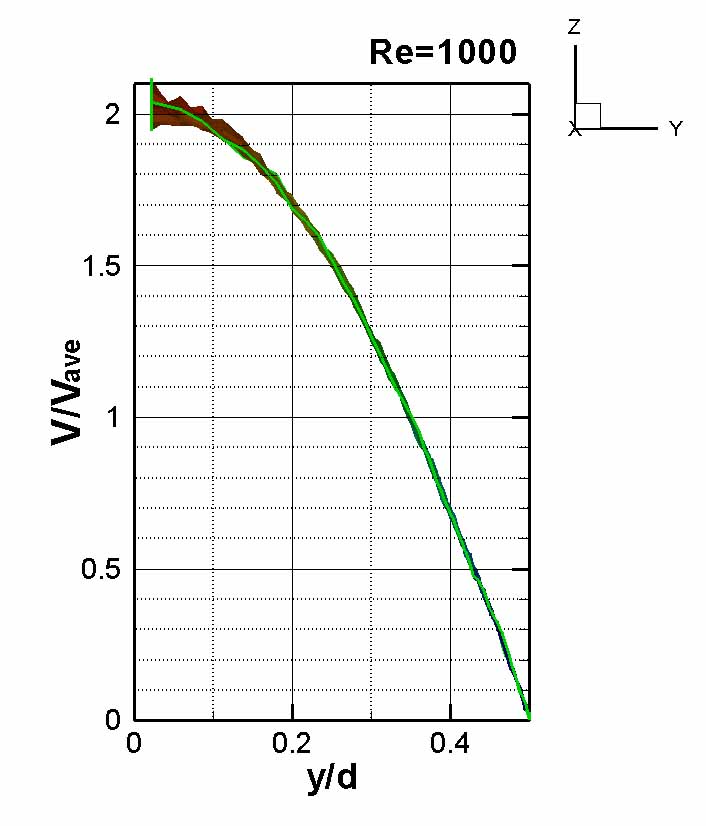
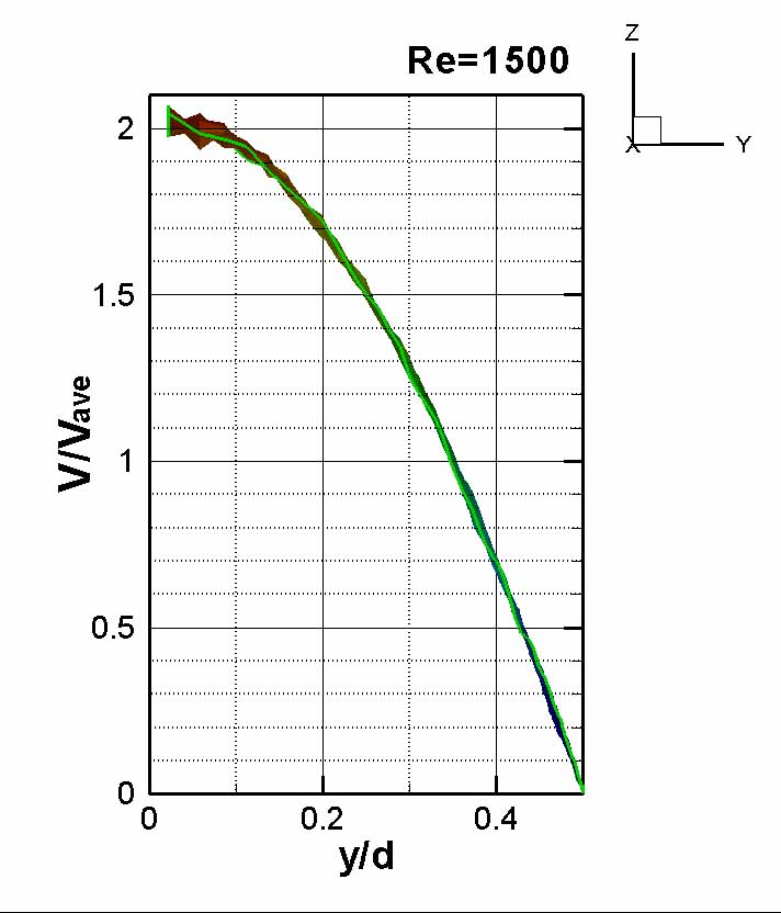
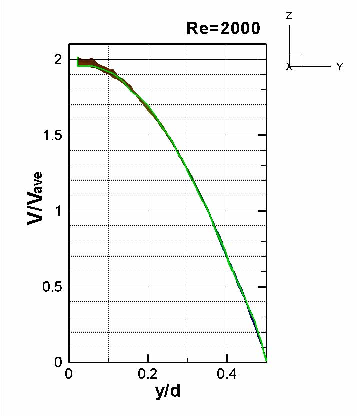
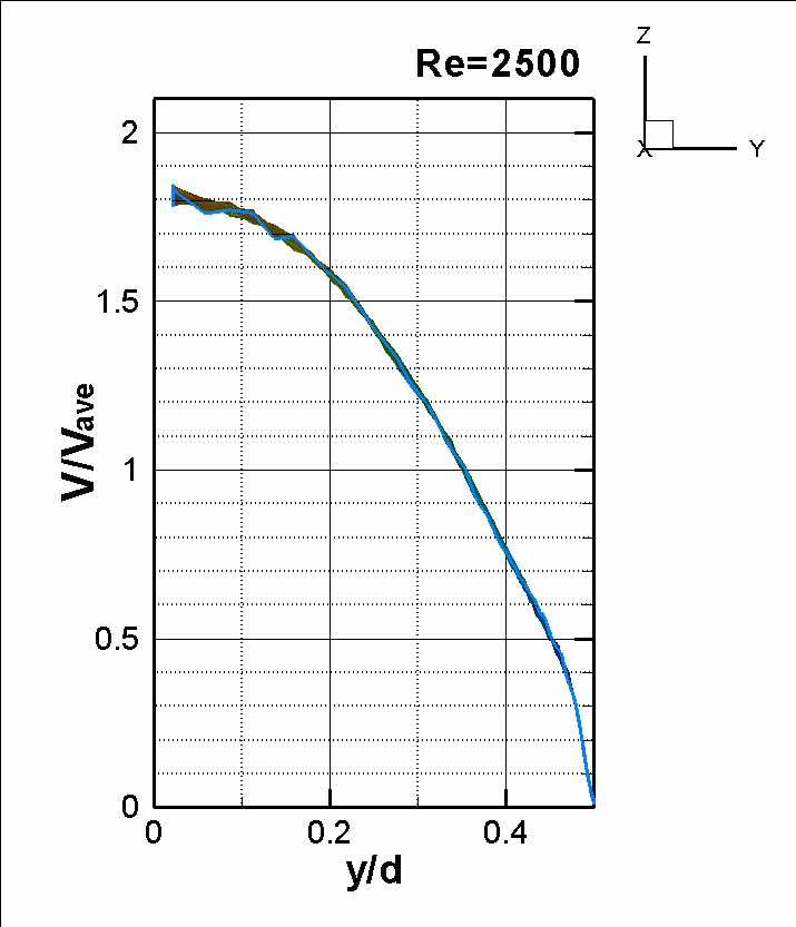
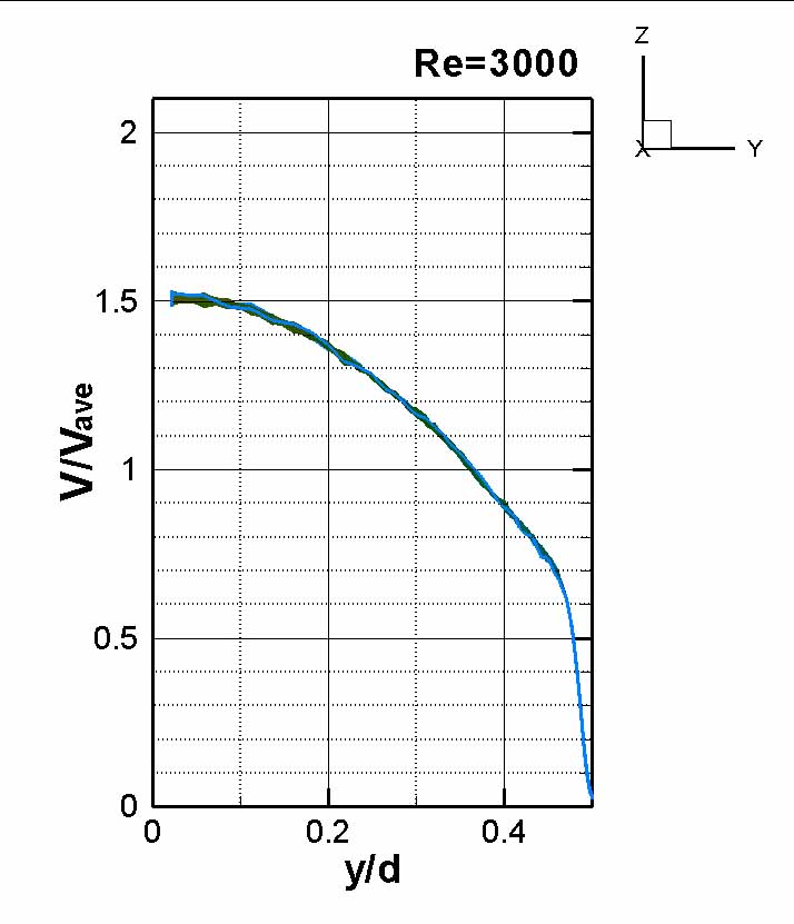
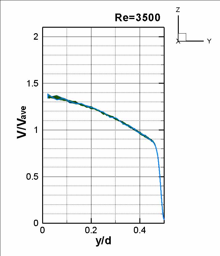
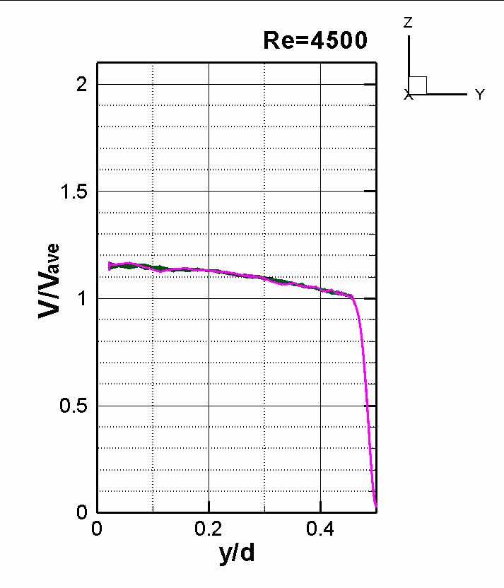
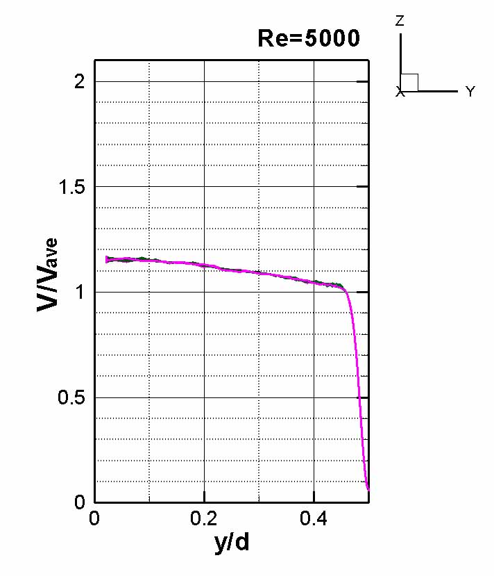
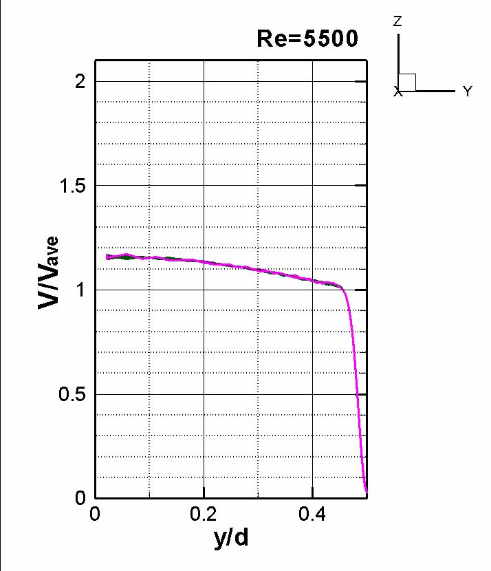
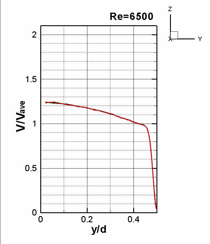
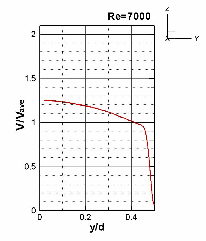
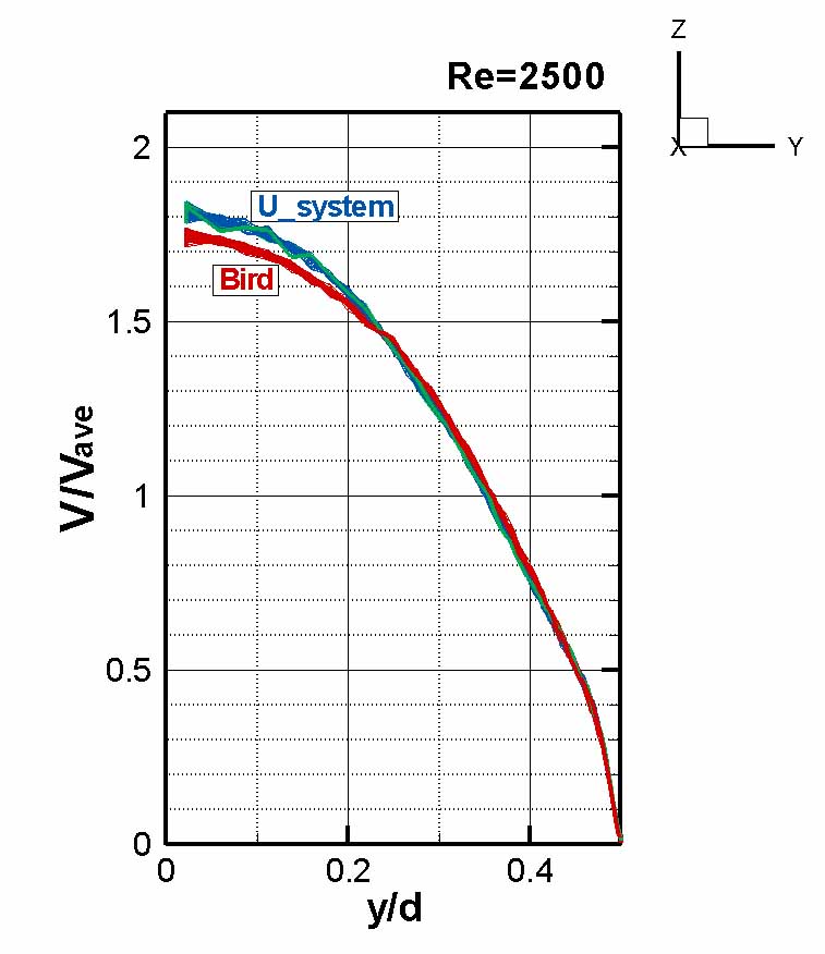
Figure 8~20 は,Re=1000~7000(平均流速は,おおよそ 10~70 m/s)で得られた管内流速の定常状態到達後の分布を,500 おきに描いたものである.また,Figure 21 は,それらをコマ送りで描いたものである.図はすべて平均流速で無次元化している.なお,Re=2500~7000 は,45ステップでの平均であるが,平均流速の小さい状態では,特に菅の中心付近で変動が大きくなるので,Re=1500と2000では,90ステップでの平均を,Re=1000 では,180ステップでの平均によって平滑化している.低速で変動が大きくなる理由は,DSMC法が分子速度(最大確率速さが約 350m/s)を基盤に解析されるためである.Re=1000~2000 は層流を示す放物線分布であり,Re=2500~3500 は,層流から乱流への遷移を示しており,Re=4000~7000 で,ほぼ乱流分布に達したと言うことができる.ただし,Re=6500 と 7000 の速度分布は,他の乱流分布から離れ始めている.この理由が,今回の計算方法における欠陥なのか,あるいは流速が大きくなり過ぎて圧縮性の影響が出てきたためなのか等のことは,今後検討すべき課題である.なお先に述べたように,修正Bird法(Bird法も同じ)では,Re数が小さくなると,結果が Usys法からずれてくる.一例として,Figure 22 に,Re=2500 における比較を示しておく.


先に述べたように,使用した3つのパラメータについては,今回の値を使用せずに,これを変えてもっと望ましい乱流・層流分布を得ることも,言い換えれば,別の境界層厚さについて挑戦することも可能であろうし,さらに,新たなパラメータを追加してより現実により近い管内流速分布を導くこともできるかも知れない.しかしそのためには,大変面倒で大がかりな繰返し計算の調査が必要となるであろう.
管内流速における乱流と層流の存在とその遷移について,著者は,元来,単純な数学で導くことのできる層流が基本にあって,何らかの原因により,そこから乱流が生み出されると考えていた.しかし,今回のDSMC計算を行って言えることであるが,「流れは本来乱流であり,それが何らかの理由で乱流成分が打ち消されて層流が作られる」と考えた方が自然のように思われる.さらに,層流の方が,DSMC計算で用いる「セル」は小さいことが要求される.これらのことをどう解釈するかは,今後の読者諸君の考察に任せたい.
(The following text is still under construction and may be revised in the future. Due to the author’s health reasons, completion is expected around autumn.)
[NEW] 3.3 DSMC Calculation of Velocity Distribution in a Circular Tube (Turbulent and Laminar Flow) (A New Attempt in 2026)
In sections 3.1 and 3.2 of this website, we discussed the possibilities of DSMC calculations of turbulent velocity distribution in a circular tube, conducted two years ago in 2024. However, several problems remained unresolved. Specifically, (a) To obtain the turbulent velocity distribution, local velocity peaks were generated at multiple distant locations near the wall, and the resulting Rayleigh-Taylor instability was used to induce a turbulent state throughout the tube. However, in actual flow, such velocity peaks are not scattered at multiple distant locations near the wall. (b) The wall roughness was approximated by a blunt saw blede shape. However, when changing the spacing and angle of the saw blede according to the Reynolds number Re, a physically meaningless approximation formula was created to handle the change. However, it is desirable to use numerical values that can explain the physical meaning, or constant values that do not depend on the Re number. (c) Although the discussion has been limited to calculations using the Usys method, it is necessary to add an explanation regarding the Bird method.
This time, in Section 3.3, we will first explain the improved calculation method and show the calculation results, and then in Section 3.4, we will release the software and explain how to use it. The range of the Re number is 1000 to 7000, as before, and the Re number is generated by changing the average flow velocity. Also, the target gas, the size of the calculation domain, and the use of periodic boundaries upstream and downstream of the tube are the same. Matters that remain unchanged from those already mentioned in Sections 3.1 and 3.2 are omitted here, so please read this explanation after familiarizing yourself with those sections.
(a) A method to avoid creating velocity peaks at multiple distant locations near the wall.
This was relatively easy to achieve. In other words, instead of fixing the saw blade shape to a single point, it is slowly moved in the direction of flow. However, moving it too quickly will disrupt the turbulent structure, so in this case, we decided to move the saw blade spacing in 45 steps. Here, one step means 200 times (220 μs) the time step Δtm (DTM = 1.1 μs) that separates molecular movement and intermolecular collisions in this DSMC calculation. Note that the saw blade spacing changes in proportion to the average flow velocity (i.e., in proportion to the Re number), so the amount of saw blade shape movement in one step differs depending on the Re number. Also, in this case, the data will be distorted unless the average of the intermediate output results is taken every 45 steps. The intermediate results are averaged in groups of 15 steps, and then three of these are combined to form one result. That is, the first time it is the average of steps 1 to 45, the second time it is the average of steps 16 to 60, and so on, and the calculation is repeated. Note that the intermediate large file created during the calculation is saved in the subfolder DATx, but it is automatically deleted when it is no longer needed. Furthermore, when molecules are reflected from the wall, the shape of the saw blade in motion is subjected to a fluctuation (perturbation) of 1/30 of the tube length (length of the computational domain) around its position at that moment.
(b) Method for approximating wall roughness with a blunt saw blade shape (saw blade spacing and blade angle)
Regarding the saw blade spacing, a value proportional to the average flow velocity was used (it is also proportional to the Re number). That is, the ratio of the tube length (a value close to the tube diameter as a characteristic length) to the saw blade spacing is made equal to the ratio of the maximum probabilistic speed of the molecules to the average flow velocity multiplied by a certain coefficient. This can be said to be a physically reasonable assumption. In the specific program, after finding the ratio of the maximum probabilistic speed to the average flow velocity, the saw blade spacing is obtained by multiplying it by a coefficient of 1.39, rounding it down to an integer (truncating), and then dividing the tube length by this value. It has been found that the boundary layer thickness can be adjusted by changing this coefficient. Although the actual wall shape should not change according to the Re number, the complex wall shape in reality encompasses many different saw blede spacings, and if we consider that the saw blede spacing corresponding to the Re number resonates and works in harmony, then the above assumptions about wall roughness can be explained. The blade angle is constant regardless of the Re number, and in this case, it is set to 35 degrees. The improved calculation method this time made it possible to keep the blade angle constant. However, even this may not be necessary if we consider that many different angles exist in actual wall roughness, and only the angle that resonates with the flow velocity appears on the surface. Since periodic boundaries are used upstream and downstream of the tube, the number of saw bledes must be limited to an integer. Therefore, the tube length changes slightly depending on the Re number, and it becomes impossible to make it equal to the tube diameter (characteristic length), which is the original setting. In this case, the decimal part was truncated to an integer, so the length of the flow field (tube length) becomes slightly shorter than the characteristic length depending on the Re number.
(c) Turbulence Calculation Using the Bird Method
In the previous explanation in Section 3.1, further explanation was omitted because the Bird method cannot strictly calculate the parabolic distribution of laminar flow. This time, we have added Pareschi et al.’s method of exact conservation of momentum and energy to the conventional Bird method, which we will call the “modified Bird method,” and investigated its application to the analysis of flow velocity in a circular tube.
In the following calculations, to obtain reasonable results in the Re number range of 1000 to 7000, the coefficient for the saw blede spacing was set to 1.39, the saw blede angle to 35 degrees, and the fluctuation width of the saw blede shape to 1/30 of the tube length (calculation domain length). These are referred to as the “three parameters.” Changing the coefficient 1.39 can change the boundary layer thickness, but remember that to obtain good results over a wide range of Re numbers using the changed value, it is necessary to carefully select the other parameters.
3.3.1 Calculation at Re=5500
First, calculations were performed at Re=5500. Figures 1 and 2 show the passage of time (video) of the flow velocity distribution in the tube. The initial flow velocity distribution was calculated by randomly determining molecular velocities from the laminar parabolic flow distribution, and the changes until the turbulent flow velocity distribution is completed are calculated. Note that the number of cells in this calculation is approximately 1.03 million, and the number of molecules is approximately 15.3 million (the number of molecules also changes slightly depending on Re because the size of the calculation domain changes depending on the Re number). Since random numbers are used to determine the initial molecular velocities, it should be noted that calculating the average flow velocity, i.e., the Re number, based on this may not necessarily result in the presise desired Re number value. The first result output is obtained after 45 steps (the time step Δtm separating molecular movement and intermolecular collisions is 1.1 μs, which is 200 times that and then 45 times again, i.e., 9.9 ms, but since it is the average value during that time, it represents the result at approximately 5 ms). Subsequent outputs are the average of three outputs obtained every 15 steps from that point, all of which are dimensionless using the average velocity.
Figures 3 and 4 show the density distribution (number density distribution) and temperature distribution obtained from the start of the calculation until the turbulence distribution was completed, respectively. Both are dimensionless using the initial density and initial temperature. While the overall flow field changes are limited to 1% to 2% for both, the density near the wall shows a change of about 5% due to the unique wall reflection processing.
Figure 5 shows the results calculated using a diffuse reflecting surface (scattered reflecting surface), and the result is a perfect parabolic distribution (laminar velocity distribution). In this case, a uniform distribution with a constant mean velocity was used as the initial distribution for the calculation.
Figure 6 shows the turbulent velocity distribution obtained using the modified Bird method. The computation time for the modified Bird method in this DSMC calculation is only about 70% of that of the Usys method, making it very fast, and the results are almost identical to those of the Usys method, making it superior in that sense (the modified Bird method was used for accuracy, but the results were the same even with the simple Bird method). However, when the laminar velocity distribution is obtained using the modified Bird method on a diffuse reflecting wall (without wall roughness), the result is as shown in Figure 7, and a perfect parabolic distribution cannot be obtained. Furthermore, even with wall roughness, the difference from the Usys method becomes slightly more apparent as the Re number decreases. The difference between the Usys method and the modified Bird method is that “the cells dividing the space appear to be smaller,” so it may be said that the cells do not need to be so fine for calculating the turbulent velocity distribution. However, considering that sufficient results cannot be obtained for the laminar velocity distribution, it seems that there is something lacking in the modified Bird method (the same is true for the conventional Bird method). In other words, unless the reason is clearly explained, the doubt that the modified Bird method cannot be reliably used cannot be dispelled.
3.3.2 Velocity distribution at Re=1000–7000
Figures 8-20 show the distribution of tube flow velocity after reaching a steady state, obtained at Re=1000-7000 (average flow velocity approximately 10-70 m/s), plotted at intervals of 500. Figure 21 shows these distributions frame by frame. All figures are dimensionless using the average flow velocity. Note that for Re=2500-7000, the average is over 45 steps, but since fluctuations are particularly large near the center of the tube at low average flow velocities, the average for Re=1500 and 2000 is over 90 steps, and for Re=1000, it is over 180 steps for smoothing. The reason for the large fluctuations at low velocities is that the DSMC method is based on molecular velocity (maximum probability velocity is approximately 350 m/s). The velocity distribution for Re = 1000 to 2000 is a parabolic distribution indicating laminar flow, Re = 2500 to 3500 indicates a transition from laminar to turbulent flow, and Re = 4000 to 7000 can be said to have almost reached a turbulent distribution. However, the velocity distributions for Re = 6500 and 7000 are beginning to deviate from the other turbulent distributions. Whether this is due to a flaw in the calculation method used, or because the flow velocity became too large and the effects of compressibility came into play, is a matter that needs to be investigated in the future. As mentioned earlier, in the modified Bird method (and the Bird method as well), the results deviate from the Usys method as the Re number decreases. As an example, Figure 22 shows a comparison at Re = 2500.
As mentioned earlier, regarding the three parameters used, it would be possible to obtain a more desirable turbulent/laminar flow distribution by changing these values, or in other words, by trying different boundary layer thicknesses. Furthermore, it might be possible to derive a tube velocity distribution closer to reality by adding new parameters. However, this would require extremely tedious and extensive iterative calculations.
Regarding the existence and transition of turbulence and laminar flow in tube velocity, the author originally believed that laminar flow, which can be derived using simple mathematics, is fundamental, and that turbulence is generated from it due to some cause. However, as can be said from this DSMC calculation, it seems more natural to think that “the flow is inherently turbulent, and for some reason the turbulent component is canceled out to create laminar flow.” Furthermore, laminar flow requires smaller “cells” used in DSMC calculations. How to interpret these points is left to the consideration of future readers.