(The following description is a preliminary version. Although I am currently refining the program and re-running the calculations, the results themselves remain virtually unchanged from those in the preliminary version. The latest version is scheduled for release around this autumn.)
[NEW] 3.3(e) DSMC Calculation of Velocity Distribution in a Circular Tube (Turbulent and Laminar Flow) (A New Attempt in 2026)
Two years ago, in 2024, sections 3.1 and 3.2 of this website discussed the possibility of DSMC calculations for turbulent velocity distributions in circular tubes, but several problems remained to be resolved. However, several problems remained unresolved. Specifically, (a) To obtain the turbulent velocity distribution, local velocity peaks were generated at multiple distant locations near the wall, and the resulting Rayleigh-Taylor instability was used to induce a turbulent state throughout the tube. However, in actual flow, such velocity peaks are not scattered at multiple distant locations near the wall. (b) The wall roughness was approximated by a blunt saw blede shape (Usami’s pseudo-surface roughness in the DSMC method). However, when changing the spacing and angle of the saw blede according to the Reynolds number Re, a physically meaningless approximation formula was created to handle the change. However, it is desirable to use numerical values that can explain the physical meaning, or constant values that do not depend on the Re number. (c) Although the discussion has been limited to calculations using the Usys method, it is necessary to add an explanation regarding the Bird method.
This time, in Section 3.3, we will first explain the improved calculation method and show the calculation results, and then in Section 3.4, we will release the software and explain how to use it. The range of the Re number is 1000 to 7000, as before, and the Re number is generated by changing the average flow velocity. Also, the target gas, the size of the calculation domain, and the use of periodic boundaries upstream and downstream of the tube are the same. Matters that remain unchanged from those already mentioned in Sections 3.1 and 3.2 are omitted here, so please read this explanation after familiarizing yourself with those sections.
(a) A method to avoid creating velocity peaks at multiple distant locations near the wall.
This was relatively easy to achieve. In other words, instead of fixing the saw blade shape to a single point, it is slowly moved in the direction of flow. However, moving it too quickly will disrupt the turbulent structure, so in this case, we decided to move the saw blade spacing in 45 steps. Here, one step means 200 times (220 μs) the time step Δtm (DTM = 1.1 μs) that separates molecular movement and intermolecular collisions in this DSMC calculation. Note that the saw blade spacing changes in proportion to the average flow velocity (i.e., in proportion to the Re number), so the amount of saw blade shape movement in one step differs depending on the Re number. Also, in this case, the data will be distorted unless the average of the intermediate output results is taken every 45 steps. The intermediate results are averaged in groups of 15 steps, and then three of these are combined to form one result. That is, the first time it is the average of steps 1 to 45, the second time it is the average of steps 16 to 60, and so on, and the calculation is repeated. Note that the intermediate large file created during the calculation is saved in the subfolder DATx, but it is automatically deleted when it is no longer needed. Furthermore, when molecules are reflected from the wall, the shape of the saw blade in motion is subjected to a fluctuation (perturbation) of 1/30 of the tube length (length of the computational domain) around its position at that moment.
(b) Method for approximating wall roughness with a blunt saw blade shape (saw blade spacing and blade angle)
Regarding the saw blade spacing, a value proportional to the average flow velocity was used (it is also proportional to the Re number). That is, the ratio of the tube length (a value close to the tube diameter as a characteristic length) to the saw blade spacing is made equal to the ratio of the maximum probabilistic speed of the molecules to the average flow velocity multiplied by a certain coefficient. This can be said to be a physically reasonable assumption. In the specific program, after finding the ratio of the maximum probabilistic speed to the average flow velocity, the saw blade spacing is obtained by multiplying it by a coefficient of 1.39, rounding it down to an integer (truncating), and then dividing the tube length by this value. It has been found that the boundary layer thickness can be adjusted by changing this coefficient. The actual wall shape should not change depending on the Reynolds number; however, this point is considered as follows. The “Usami’s pseudo-surface roughness” proposed here simulates the highly complex nature of actual surface roughness using a simple sawtooth profile. Given that actual wall geometries feature a wide range of sawtooth spacings, yet -for a specific Reynolds number (or mean flow velocity)- only a particular spacing resonates and influences the fluid, it is reasonable to scale the sawtooth width in proportion to the mean flow velocity in order to apply this simplified approximation across a broad range of Reynolds numbers. The blade angle is constant regardless of the Re number, and in this case, it is set to 35 degrees. The improved calculation method this time made it possible to keep the blade angle constant. However, even this may not be necessary if we consider that many different angles exist in actual wall roughness, and only the angle that resonates with the flow velocity appears on the surface. Since periodic boundaries are used upstream and downstream of the tube, the number of saw bledes must be limited to an integer. Therefore, the tube length changes slightly depending on the Re number, and it becomes impossible to make it equal to the tube diameter (characteristic length), which is the original setting. In this case, the decimal part was truncated to an integer, so the length of the flow field (tube length) becomes slightly shorter than the characteristic length depending on the Re number.
(c) Turbulence Calculation Using the Bird Method
In the previous explanation in Section 3.1, further explanation was omitted because the Bird method cannot strictly calculate the parabolic distribution of laminar flow. This time, we have added Pareschi et al.’s method of exact conservation of momentum and energy to the conventional Bird method, which we will call the “modified Bird method,” and investigated its application to the analysis of flow velocity in a circular tube.
In the following calculations, to obtain reasonable results in the Re number range of 1000 to 7000, the coefficient for the saw blede spacing was set to 1.39, the saw blede angle to 35 degrees, and the fluctuation width of the saw blede shape to 1/30 of the tube length (calculation domain length). These are referred to as the “three parameters.” Changing the coefficient 1.39 can change the boundary layer thickness, but remember that to obtain good results over a wide range of Re numbers using the changed value, it is necessary to carefully select the other parameters.
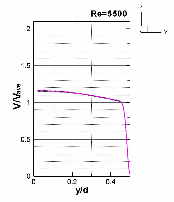
3.3.1 Calculation at Re=5500
First, calculations were performed at Re=5500. Figures 1 and 2 show the passage of time (video) of the flow velocity distribution in the tube. The initial flow velocity distribution was calculated by randomly determining molecular velocities from the laminar parabolic flow distribution, and the changes until the turbulent flow velocity distribution is completed are calculated. Note that the number of cells in this calculation is approximately 1.03 million, and the number of molecules is approximately 15.3 million (the number of molecules also changes slightly depending on Re because the size of the calculation domain changes depending on the Re number). Since random numbers are used to determine the initial molecular velocities, it should be noted that calculating the average flow velocity, i.e., the Re number, based on this may not necessarily result in the presise desired Re number value. The first result output is obtained after 45 steps (the time step Δtm separating molecular movement and intermolecular collisions is 1.1 μs, which is 200 times that and then 45 times again, i.e., 9.9 ms, but since it is the average value during that time, it represents the result at approximately 5 ms). Subsequent outputs are the average of three outputs obtained every 15 steps from that point, all of which are dimensionless using the average velocity.
Figures 3 and 4 show the density distribution (number density distribution) and temperature distribution obtained from the start of the calculation until the turbulence distribution was completed, respectively. Both are dimensionless using the initial density and initial temperature. While the overall flow field changes are limited to 1% to 2% for both, the density near the wall shows a change of about 5% due to the unique wall reflection processing.
Figure 5 shows the results calculated using a diffuse reflecting surface (scattered reflecting surface) with no surface roughness, and the result is a perfect parabolic distribution (laminar velocity distribution). In this case, a uniform distribution with a constant mean velocity was used as the initial distribution for the calculation.
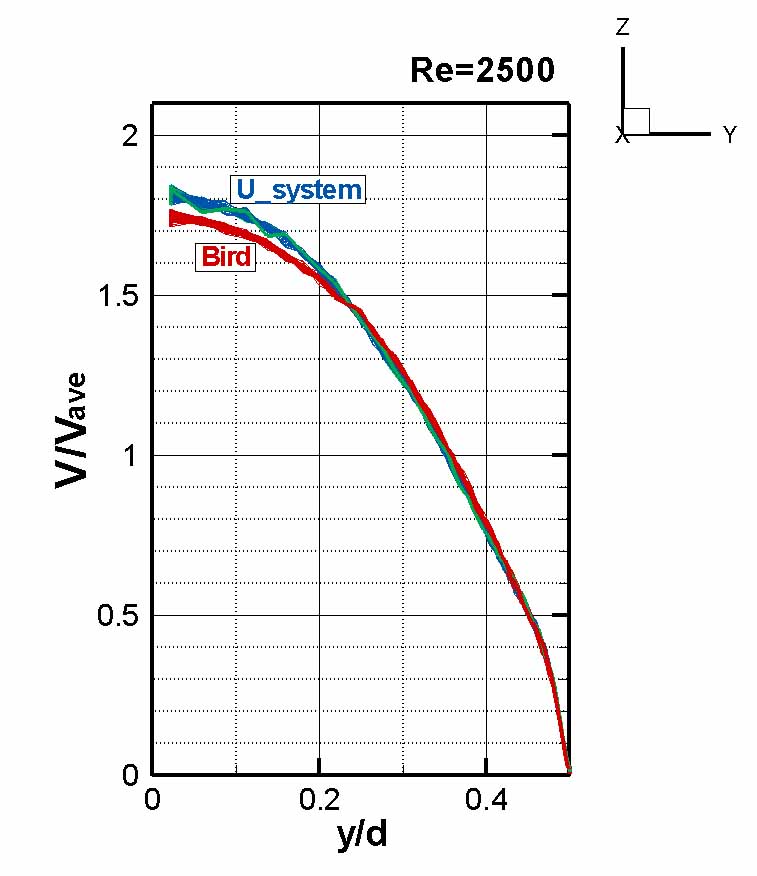
Figure 6 shows the turbulent velocity distribution obtained using the modified Bird method. The computation time for the modified Bird method in this DSMC calculation is only about 70% of that of the Usys method, making it very fast, and the results are almost identical to those of the Usys method, making it superior in that sense (the modified Bird method was used for accuracy, but the results were the same even with the simple Bird method). However, when the laminar velocity distribution is obtained using the modified Bird method on a diffuse reflecting wall (without wall roughness), the result is as shown in Figure 7, and a perfect parabolic distribution cannot be obtained. Furthermore, even with wall roughness, the difference from the Usys method becomes slightly more apparent as the Re number decreases. The difference between the Usys method and the modified Bird method is that “the cells dividing the space appear to be smaller,” so it may be said that the cells do not need to be so fine for calculating the turbulent velocity distribution. However, considering that sufficient results cannot be obtained for the laminar velocity distribution, it seems that there is something lacking in the modified Bird method (the same is true for the conventional Bird method). In other words, unless the reason is clearly explained, the doubt that the modified Bird method cannot be reliably used cannot be dispelled.
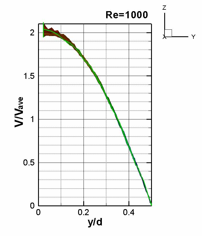
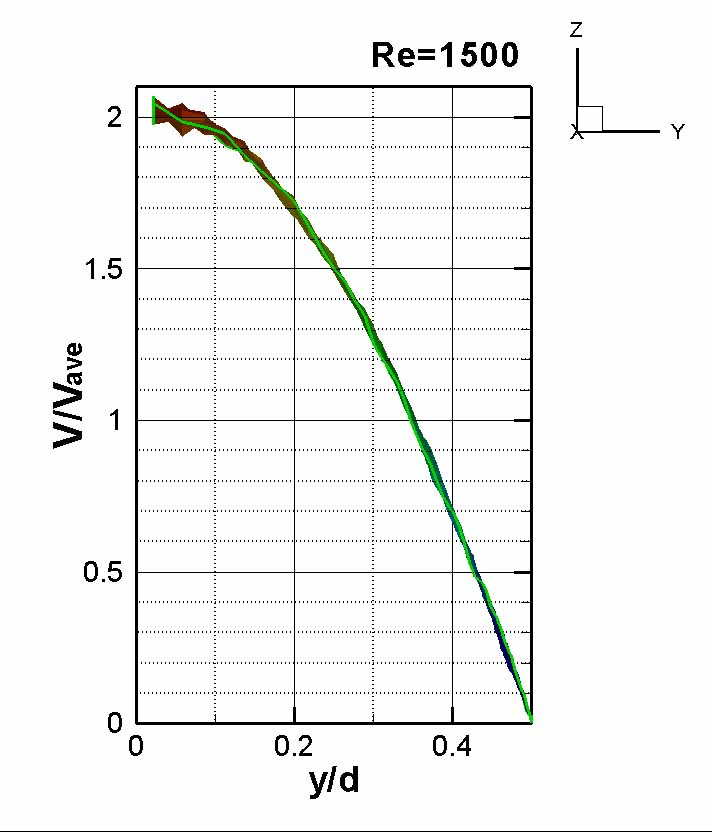
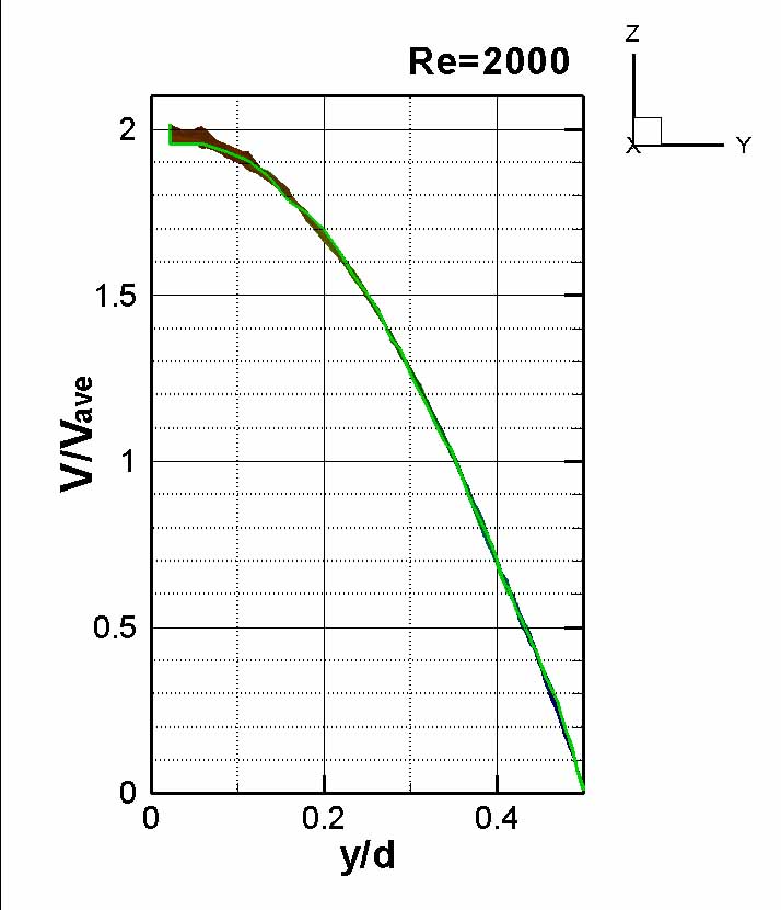
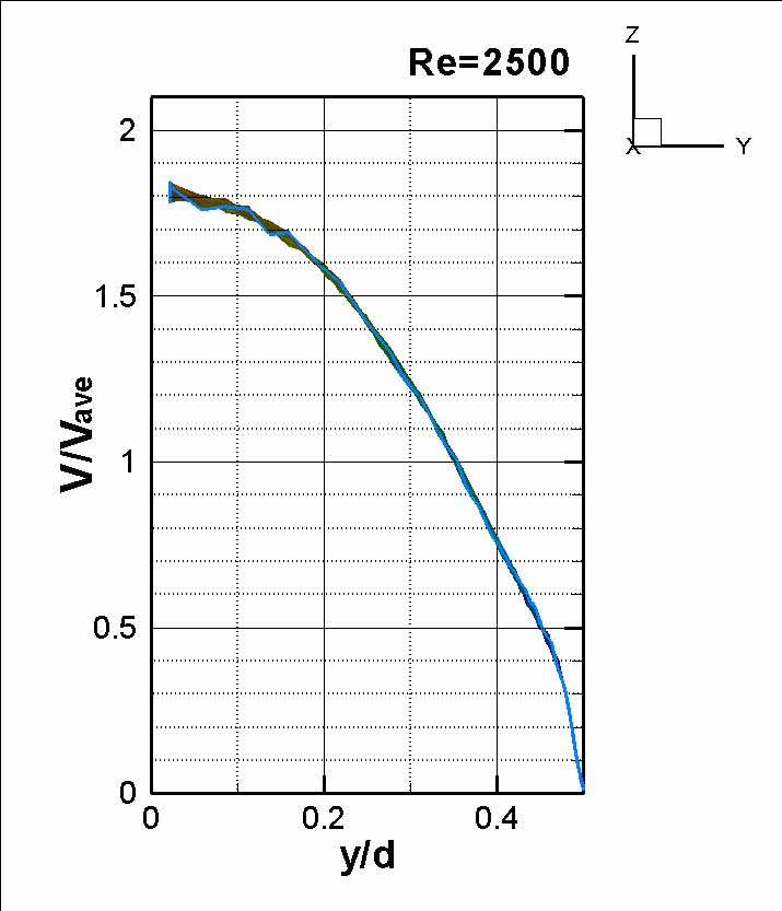
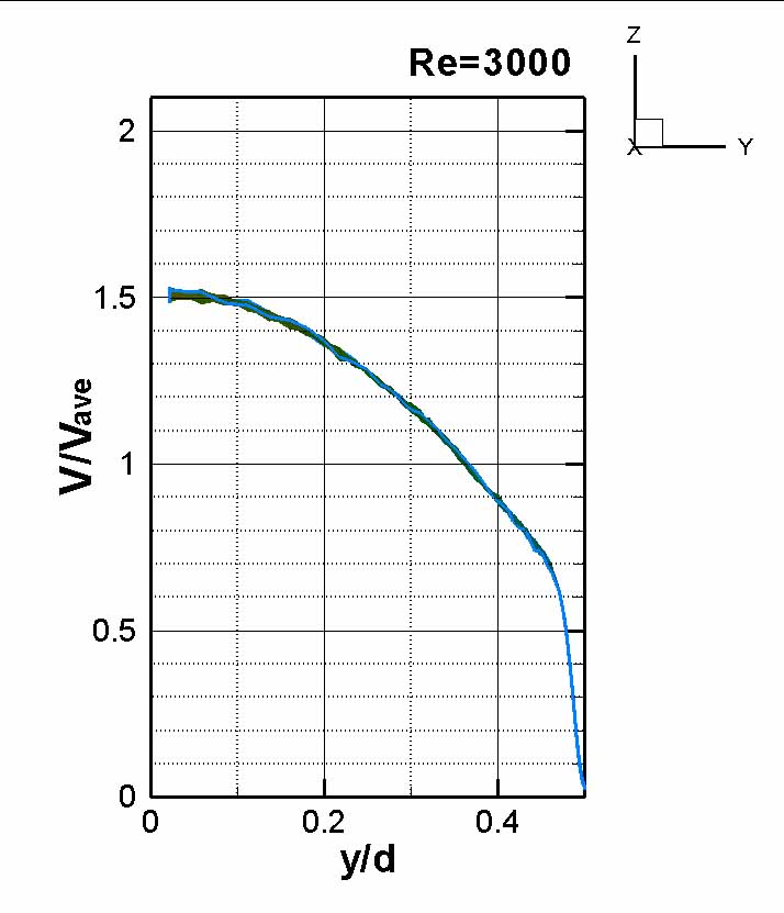
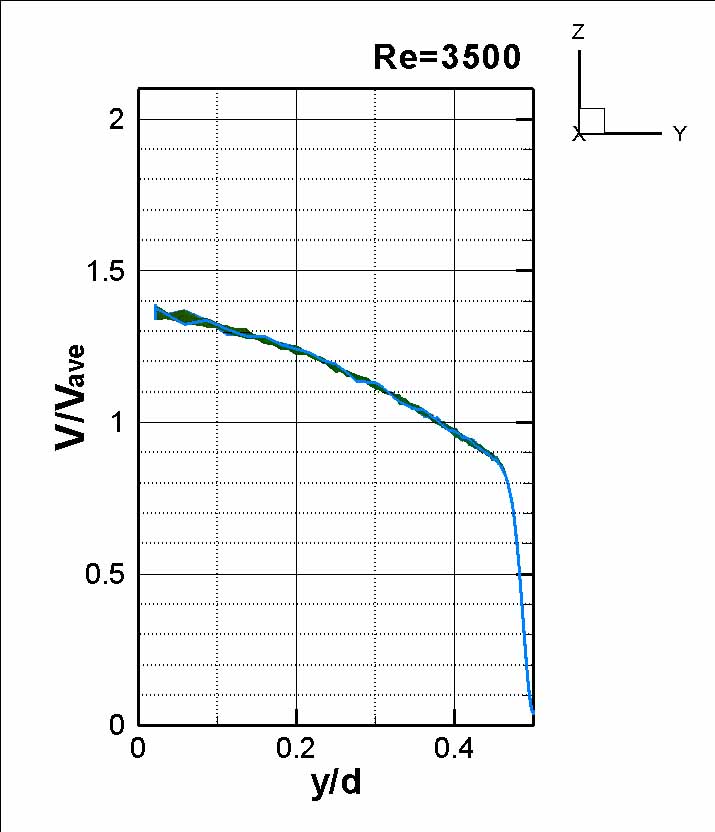
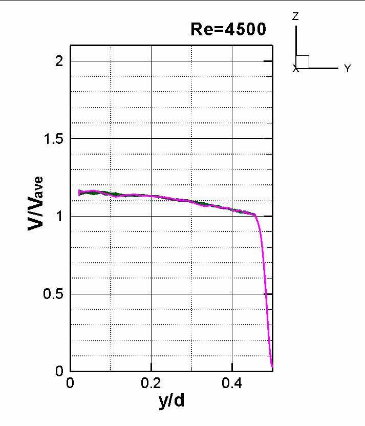
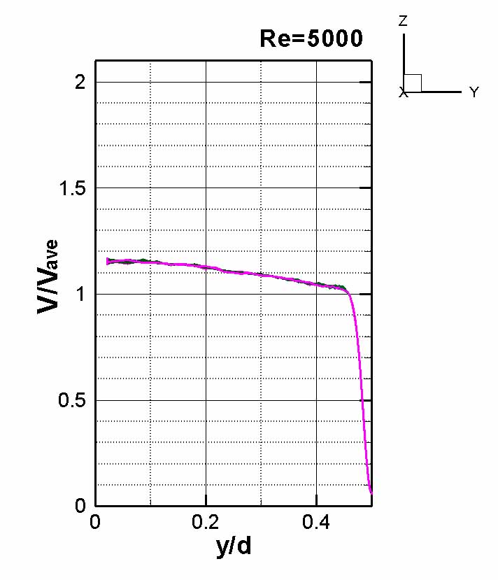
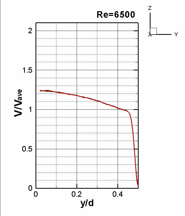
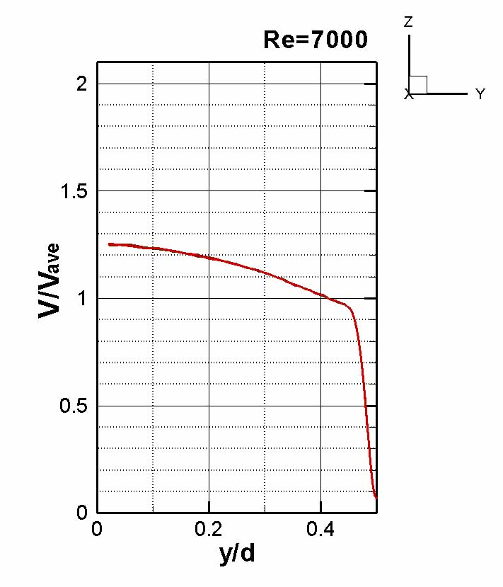
3.3.2 Velocity distribution at Re=1000–7000
Figures 8-20 show the distribution of tube flow velocity after reaching a steady state, obtained at Re=1000-7000 (average flow velocity approximately 10-70 m/s), plotted at intervals of 500. Figure 21 shows these distributions frame by frame. All figures are dimensionless using the average flow velocity. Note that for Re=2500-7000, the average is over 45 steps, but since fluctuations are particularly large near the center of the tube at low average flow velocities, the average for Re=1500 and 2000 is over 90 steps, and for Re=1000, it is over 180 steps for smoothing. The reason for the large fluctuations at low velocities is that the DSMC method is based on molecular velocity (maximum probability velocity is approximately 350 m/s). The velocity distribution for Re = 1000 to 2000 is a parabolic distribution indicating laminar flow, Re = 2500 to 3500 indicates a transition from laminar to turbulent flow, and Re = 4000 to 7000 can be said to have almost reached a turbulent distribution. However, the velocity distributions for Re = 6500 and 7000 are beginning to deviate from the other turbulent distributions. Whether this is due to a flaw in the calculation method used, or because the flow velocity became too large and the effects of compressibility came into play, is a matter that needs to be investigated in the future. As mentioned earlier, in the modified Bird method (and the Bird method as well), the results deviate from the Usys method as the Re number decreases. As an example, Figure 22 shows a comparison at Re = 2500.


As mentioned earlier, regarding the three parameters used, it would be possible to obtain a more desirable turbulent/laminar flow distribution by changing these values, or in other words, by trying different boundary layer thicknesses. Furthermore, it might be possible to derive a tube velocity distribution closer to reality by adding new parameters. However, this would require extremely tedious and extensive iterative calculations.
Regarding the existence and transition of turbulence and laminar flow in tube velocity, the author originally believed that laminar flow, which can be derived using simple mathematics, is fundamental, and that turbulence is generated from it due to some cause. However, as can be said from this DSMC calculation, it seems more natural to think that “the flow is inherently turbulent, and for some reason the turbulent component is canceled out to create laminar flow.” Furthermore, laminar flow requires smaller “cells” used in DSMC calculations. How to interpret these points is left to the consideration of future readers.