(The text in this section is the latest version, created in September 2026. Note that the older, provisional version written in June has been retained for reference at 3.3(e)′ [Old…].)
Two years ago, in 2024, Sections 3.1 and 3.2 of this website discussed the potential of using the DSMC method to calculate turbulent velocity profiles in circular tubes; however, several issues remained to be resolved. Specifically: (a) To generate a turbulent velocity profile, local velocity peaks were induced at multiple discrete locations near the wall, triggering Rayleigh-Taylor instability to drive the entire tube flow into a turbulent state; however, actual flows do not feature such scattered velocity peaks near the wall. (b) Wall roughness was approximated using a blunt sawblade shape (Usami’s pseudo-surface roughness for the DSMC method); however, the approximation formulas used to adjust the sawblade spacing and angle according to the Reynolds number (Re) lacked physical significance. It is desirable to use values with clear physical meaning or constants independent of the Reynolds number. (c) The discussion was limited exclusively to calculations using the Usys method, creating a need to also explain the Bird method.
In this section (Section 3.3), we first describe the improved calculation method and present the results. Subsequently, in Section 3.4, we will release the software and explain how to use it. As before, the Reynolds number range is set to 1,000–7,000, with specific Re values achieved by varying the mean flow velocity. The approach regarding the target gas, the size of the computational domain, and the use of periodic boundary conditions upstream and downstream of the circular tube remains the same as in the previous study. Details previously described in Sections 3.1 and 3.2 are omitted here; please ensure you are familiar with that information before reading this explanation.
(a) Method to avoid creating multiple velocity peaks at discrete locations near the wall
This was achieved relatively easily. Instead of fixing the sawblade shape at a single point, it is moved slowly in the flow direction. However, moving it too quickly disrupts the turbulent structure; therefore, we set the movement rate such that the shape traverses the distance of one sawblade interval over 45 steps. Here, one step is defined as 200 times the minimum time interval Δtm (DTM = 1.1 μs)—which separates molecular movement and intermolecular collisions in this DSMC calculation—resulting in a duration of 220 μs. Since the sawblade interval varies in proportion to the mean flow velocity (and thus the Reynolds number), the distance the shape moves in a single step depends on the Reynolds number. Furthermore, to avoid data distortion, it is essential to average the intermediate output results over the 45-step cycle. Intermediate results are averaged in 15-step increments, and three of these averaged values are combined to form a single result. Specifically, the first result is the average of steps 1–45, while the second is the average of steps 16–60, and so on. Intermediate data generated during the calculation are saved in a subfolder named “DATx”; although these are large files, they are automatically deleted when no longer needed. Additionally, when molecules reflect off the wall, the moving sawblade shape is subjected to a fluctuation (perturbation) of 1/35 of the characteristic length (tube diameter), centered on its instantaneous position.
(b) Method of approximating wall roughness using a blunt sawblade shape (sawblade spacing and blade angle)
Regarding the sawblade spacing, a value proportional to the mean flow velocity (and thus proportional to the Reynolds number) was used. In other words, the ratio of the characteristic length (tube diameter) to the sawblade spacing is set equal to the ratio of the most probable speed to the mean flow velocity, multiplied by a specific coefficient. This is considered a physically reasonable assumption. In the actual program, the sawblade spacing is determined by calculating the ratio of the most probable speed to the mean flow velocity, multiplying it by a coefficient of 1.30, and then dividing the characteristic length by this result. The tube length is calculated by multiplying the sawblade spacing by the integer part of the value obtained when dividing the characteristic length by the sawblade spacing. Note that by adjusting parameters such as this coefficient (1.30), the fluctuation (perturbation) amplitude (1/35), and the sawblade angle (35 degrees, described later), the flow velocity distribution corresponding to the Reynolds number can be tuned to differ from the results obtained in this study. Regarding the actual wall shape, while it should not change in response to the Reynolds number (Re), we approach this issue as follows. The “Usami pseudo-surface roughness”—proposed here as a “disturbance to induce turbulence”—simulates the highly complex nature of actual surface roughness using a simple sawblade profile. In a real wall, sawblade spacings vary widely; however, if we assume that for a given Reynolds number (i.e., a specific mean flow velocity), only a specific sawblade spacing resonates with that Re number to influence the fluid, then scaling the sawblade width in proportion to the mean flow velocity is not an unnatural assumption for applying this simplified approximation across a wide range of Reynolds numbers. The blade angle remains constant regardless of the Re number; in this study, it is set to 35 degrees. The improved calculation method used here allows for a constant blade angle. However, given that actual surface roughness involves a multitude of angles—and assuming that only the angle resonating with the flow velocity becomes significant—it might not actually be necessary to fix the angle; this remains a topic for future study. Since periodic boundary conditions are applied at the upstream and downstream ends of the tube, the number of sawblade blades must be an integer. Consequently, the tube length varies slightly with the Re number, making it impossible to strictly match the tube diameter (characteristic length) as originally intended. In this study, the value was truncated to an integer, resulting in a flow field length (tube length) that is slightly shorter than the characteristic length, depending on the Re number.
(c) Turbulence calculation using the Bird method
In the previous explanation in Section 3.1, further details regarding the Bird method were omitted because it cannot precisely calculate the parabolic velocity profile characteristic of laminar flow. In this study, we defined a “Modified Bird Method”—incorporating the momentum and energy conservation techniques proposed by Pareschi et al. into the conventional Bird method—and applied it to analyze the flow velocity within a circular tube.
For the calculations below, covering a Reynolds number (Re) range of 1000 to 7000, the following settings were used to ensure reasonable results: a coefficient of 1.30 for the sawblade spacing, a sawblade angle of 35 degrees, and a sawblade shape fluctuation width set to 1/35 of the tube diameter (characteristic length). These are referred to as the “three parameters.” While altering these three parameters can yield velocity distributions different from the current results in response to changes in Re, it is important to note that careful selection of these parameters is required to obtain satisfactory results across a wide Re range.
3.3.1 Calculation at Re = 5500
First, a calculation was performed at Re = 5500. Figures 1 and 2 show the time evolution of the flow velocity distribution within the tube (as an animation); the calculation began with an initial velocity distribution based on a laminar parabolic profile with randomly assigned molecular velocities, tracking the transition until a turbulent velocity profile was established. The simulation involved approximately 1.03 million cells and 13 million molecules (the number of molecules varies slightly with Re because the computational domain size changes). Note that since initial molecular velocities are determined using random numbers, the resulting average velocity—and thus the calculated Re—does not necessarily match the target Re exactly. The first output was generated after 45 steps. The minimum time interval Δtm separating molecular movement and intermolecular collisions is 1.1 μs, which is 200 times and then 45 times again, i.e., 9.9 ms, effectively corresponding to the state at approximately 5 ms. Subsequent outputs represent the average of three results obtained at 15-step intervals; all results are normalized by the average flow velocity.
Figures 3 and 4 show the density distribution (number density) and temperature distribution, respectively, obtained during the period from the start of the calculation until the turbulent flow distribution was fully established. Both distributions are normalized by the initial density and temperature. While the magnitude of the final changes in density and temperature remains below 1% throughout the flow field—excluding the region near the wall—variations of approximately 6% in density and 2% in temperature occur near the wall due to the specific wall reflection treatment employed.
Figure 5(a) shows the flow velocity distribution calculated using a diffuse reflection surface (without surface roughness); the result exhibits a nearly perfect parabolic profile (characteristic of laminar flow). However, as seen in the orange-colored region of Figure 5(b), values exceeding twice the mean flow velocity (the theoretical maximum) are sometimes observed near the central axis. Since the density near the central axis is slightly lower than the average, the flow should ideally be analyzed in terms of mass velocity (mass flux) rather than flow velocity. An analysis based on mass velocity yielded some improvement, but the overall trend remained largely unchanged (Figure 5(c)). Note that a uniform distribution based on the mean flow velocity was used as the initial distribution for these calculations.
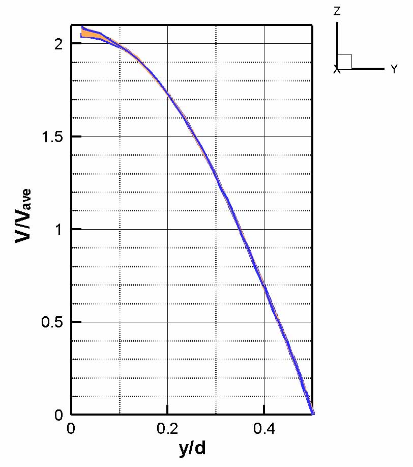
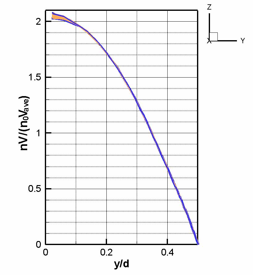
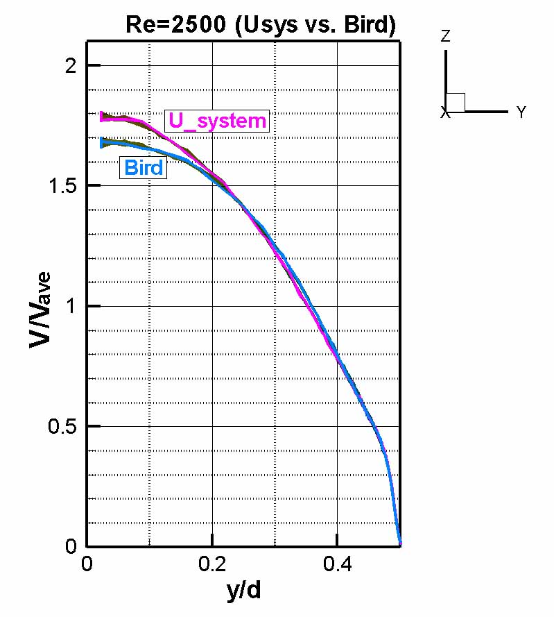
Figure 6 shows the turbulent velocity profile obtained using the modified Bird method. In this DSMC study, the modified Bird method required only about 70% of the computation time of the Usys method, allowing for faster calculation; furthermore, the results were virtually identical to those of the Usys method, making it highly advantageous in that respect (the modified Bird method was used for precision, though the standard Bird method yielded similar results). However, when the modified Bird method is applied to a diffuse reflection wall (without roughness) to determine the laminar velocity profile, the result is as shown in Figure 7, failing to produce a perfect parabolic distribution. Additionally, even with wall roughness, slight discrepancies from the Usys method emerge as the Reynolds number decreases. The key difference between the Usys method and the modified Bird method is that, in the former, the spatial cells appear effectively smaller; this might suggest that extremely fine cell resolution is not required for calculating turbulent velocity profiles. Nevertheless, the failure to obtain satisfactory results for laminar velocity profiles implies a deficiency in the modified Bird method (a limitation shared by the conventional Bird method). In short, until the underlying reason for this is clarified, one cannot fully dispel doubts regarding the reliability of the modified Bird method.
3.3.2 Velocity Profiles at Re = 1000–7000
Figures 8 through 20 show the steady-state velocity profiles within the tube for Reynolds numbers (Re) ranging from 1000 to 7000 (corresponding to mean velocities of approximately 10–70 m/s), plotted at intervals of 500. Figure 21 presents these profiles in a sequential frame-by-frame format. All figures are normalized using the mean velocity. While the profiles for Re = 3000–7000 represent averages over 45 steps, fluctuations—particularly near the tube center—increase at lower mean velocities; consequently, the data for Re = 1000, 1500 and 2000 were smoothed by averaging over 180 steps, and the data for Re = 2500 by averaging over 135 steps. If you desire smooth results even at Re ≥ 3000, it is advisable to use the average of 90 or 135 steps. The reason for the increased fluctuations at low speeds is that the DSMC method relies on molecular velocities (with a most probable speed of approximately 350 m/s) for its analysis. A parabolic profile characteristic of laminar flow appears at Re = 1000–2000; a transition from laminar to turbulent flow is observed at Re = 2500–3500; and a profile closely resembling turbulent flow is established at Re = 4000–7000. However, the velocity profiles at Re = 6500 and 7000 begin to deviate from the other turbulent profiles. Future study is required to determine whether this is due to a flaw in the current computational method—which centers on the “surface roughness approximation” I proposed—or if it results from compressibility effects arising as the flow velocity becomes excessively high. As previously mentioned, results obtained using the modified Bird method (and the standard Bird method) tend to diverge from those of the Usys method as the Reynolds number decreases; Figure 22 illustrates this comparison for Re = 2500.
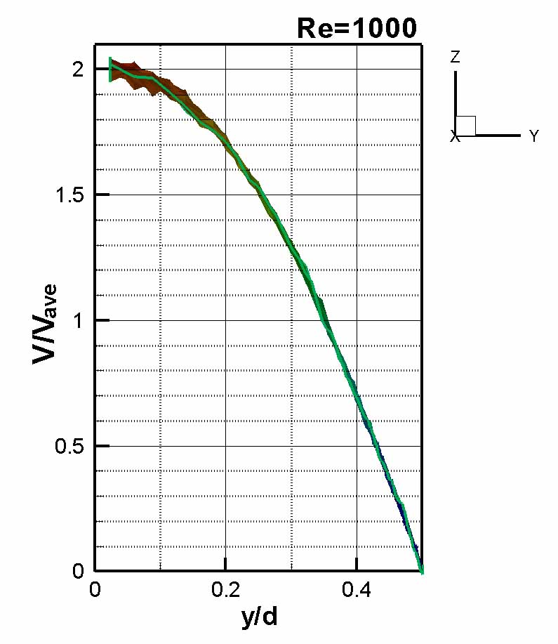
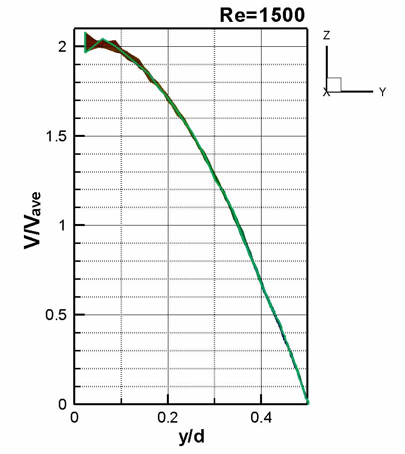
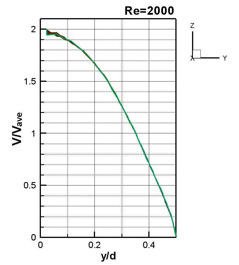
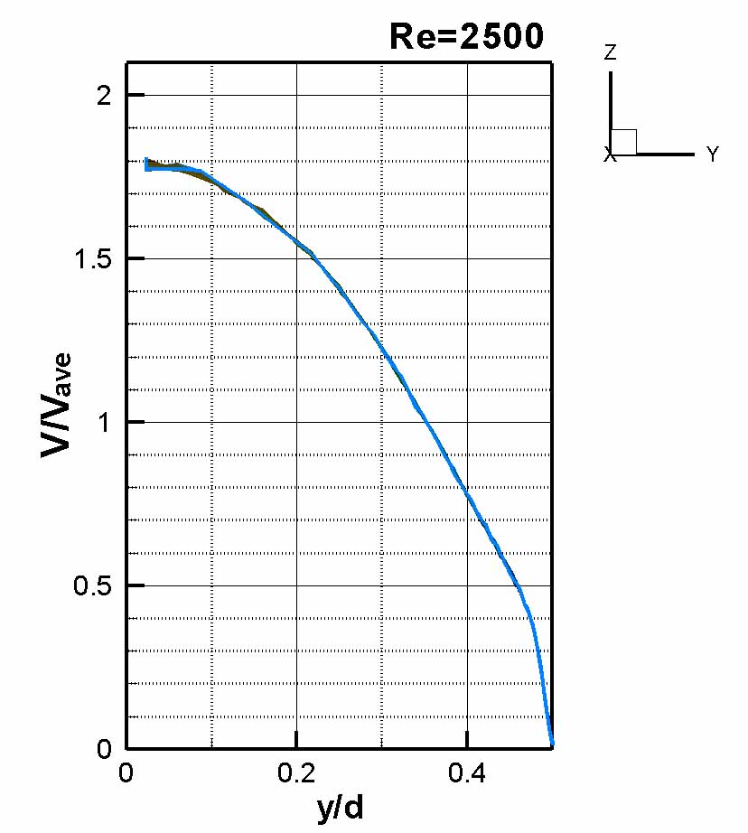
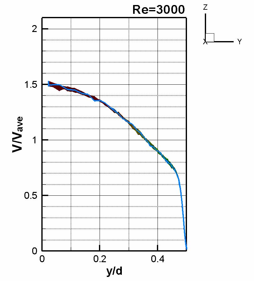
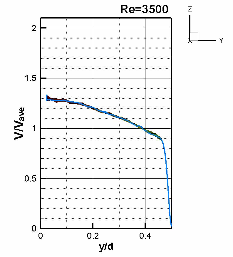
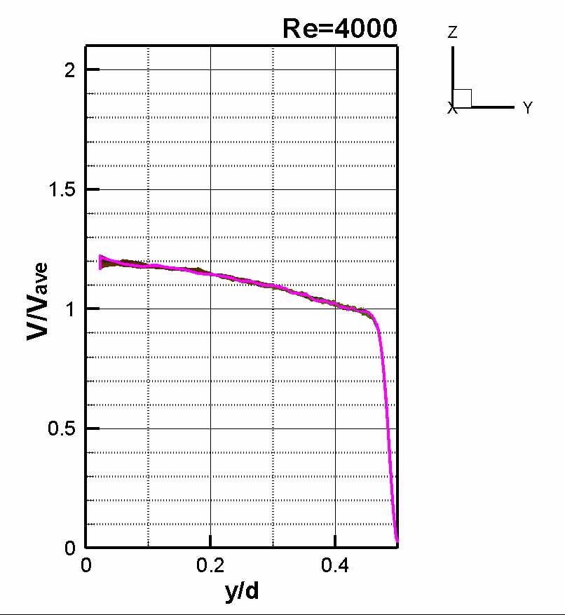
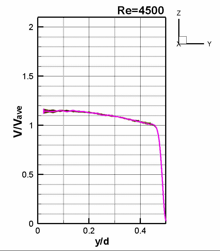
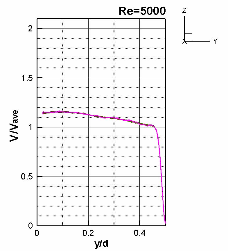
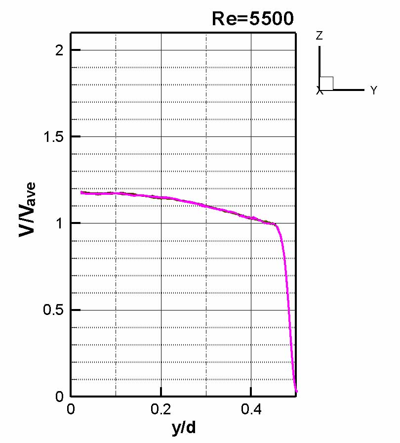
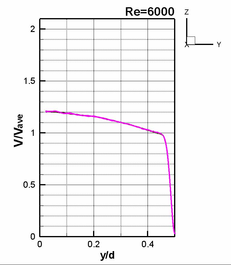
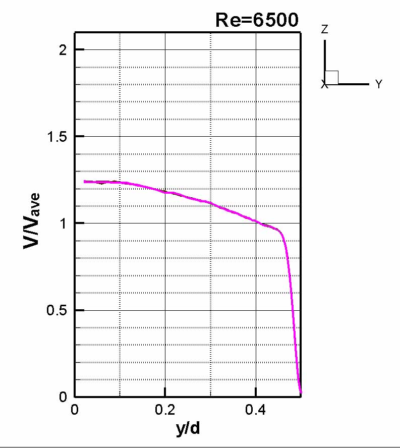
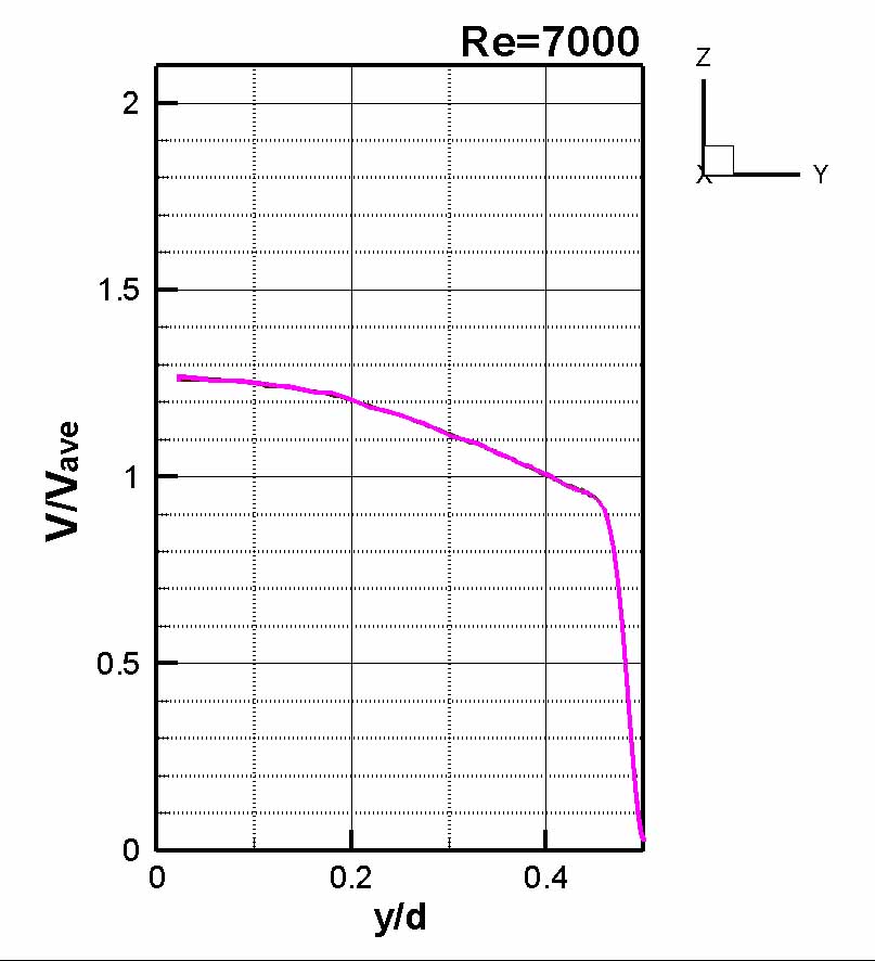
As previously mentioned, regarding the three parameters employed here, it would likely be possible to obtain more desirable turbulent and laminar distributions by varying them rather than using the current values; furthermore, introducing new parameters might allow for the derivation of in-tube velocity profiles that more closely resemble reality. However, such an endeavor would require extensive and laborious iterative calculations.
Regarding the existence of turbulent and laminar flow within the tube and the transition between them, the author initially held the view that laminar flow—which can be derived through simple mathematics—was the fundamental state, and that turbulence arose from it due to some underlying cause. However, after conducting the current DSMC simulations, I find it plausible to consider the following perspective: “Since the potential to generate Rayleigh-Taylor instability exists regardless of the magnitude of the Reynolds number (Re), the flow is inherently turbulent in nature; however, as Re decreases, inertial forces weaken to the point where vortices can no longer be sustained, causing the turbulent distribution to collapse into a laminar one.” It should also be noted that laminar flow requires smaller “cells” for DSMC calculations. I leave the interpretation of these points to the reader’s own analysis. Furthermore, as I do not have experimental data at hand to definitively assess the accuracy of the simulations, I would strongly encourage readers to investigate this matter further.
Calculating these velocity profiles requires a significant amount of time. Specifically, the time required to complete a calculation for a single Reynolds number is approximately 44 hours using a Ryzen 9 9950X3D CPU (with 32 threads; calculation times are nearly identical for the 9950X and 9950X3D2 models) and approximately 88 hours—double that duration—using a Ryzen 7 6800H (with 16 threads); these figures assume the use of an M.2 SSD in both cases. When using the 9950X3D for DSMC calculations, a high-performance graphics card is unnecessary, and air cooling suffices for the CPU (in the author’s experience, inexpensive all-in-one liquid cooling systems actually yield poorer performance, suffer from slow thermal response, and are prone to failure). Although the Ryzen 7 6800H was released some time ago, it offers excellent price-to-performance; as a laptop processor, it consumes little power while delivering strong performance (At the end of 2025, a CPU with nearly identical performance—the Ryzen 7 170—was released; while its performance is slightly lower, apparently, it consumes less power). However, because the workload involves intensive, long-duration calculations, a robust laptop is required. In the author’s case, using a 16-inch Lenovo laptop with the display turned off resulted in a power consumption of approximately 80 W during calculation (Make sure to clean the air intake for air cooling with a vacuum cleaner at least once a month.).