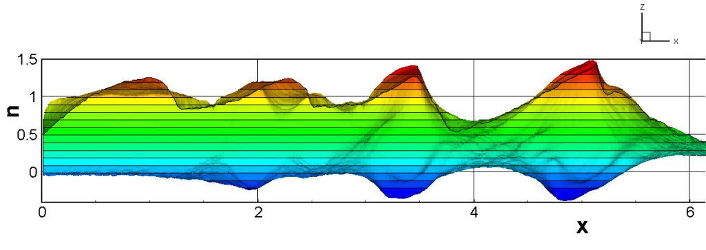
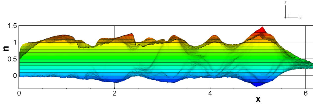
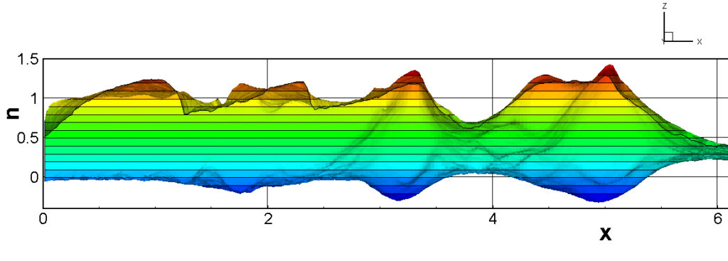
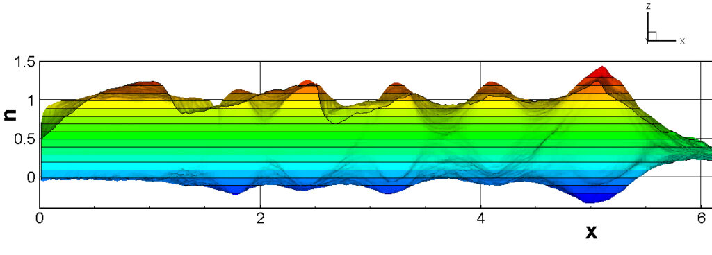
Although Chapter 4 is titled “Analysis of Turbulence in Supersonic Jets,” in reality, we use a program that is basically the same as the one used in the test (trial) calculation in Chapter 2. That is, the flow starts from a virtual stagnation point set to the upstream pressure, passes through a circular orifice, and then forms a supersonic jet and flows downstream. The initial condition downstream of the orifice is at rest with downstream back pressure. However, in the test calculation in Chapter 2, coarse spatial cells and extremely large time steps were used so that the calculations could be completed in a relatively short time even on a small PC, and as illustrated in “5.1(e) Overview of the DSMC Method”, the space upstream of the orifice is omitted. On the other hand, in Chapter 4, the size of the spatial cells is made as close as possible to the local mean free path, and the time step is made as close as possible to the mean free time (mean collision time) of the molecules so that the turbulent shape of the jet can be reproduced. Of course, if the pressure is close to atmospheric pressure, it is impossible to match the mean free path or mean free time. As such, the calculations in Chapter 4 are serious, so a reasonably fast PC is required, and 32GB of memory is required (16GB is possible for some calculations). By the way, in my case, I mainly use a CPU (AMD3990x with 128 threads) that can execute two independent calculations at the same time using each 64 threads, but even so, it takes days to complete a calculation under any condition (a comparison of calculation times for different CPUs has been shown at the end of Chapter 2). Calculations with a large pressure ratio will end relatively quickly because the total number of molecules is smaller, and the smaller the upstream pressure, the sooner it will end. In addition, a large amount of intermediate data uvw333 (all data on the position coordinates and velocity components of molecules, up to a maximum of about 500 million) is output from time to time, so a high-speed SSD is also required. In addition, in the test calculations in Chapter 2, the ratio of the upstream pressure to the downstream pressure (pressure ratio) was fixed at 50, but in Chapter 4, the pressure ratio can be changed from 2 to 16. Note that the pressure ratio is limited to 16 because it is necessary to keep the calculation area small, as it is thought that the turbulence of the jet will not increase at a pressure ratio higher than this. The upstream stagnation pressure (absolute pressure) can vary from 1mmHg to 760mmHg (1 atm). For a supersonic jet, one might think that the upstream pressure should be larger. However, if the upstream pressure is large enough that the flow condition is considered to be a continuum flow region, it is fine to assume that the jet shape is determined only by the pressure ratio. The DSMC method was originally devised for the analysis of rarefied gases, and its calculation limit pressure is set to a little over 1 atm (there is no limit on the lower pressure). The target is a simple argon gas. The question of why air or fuel gases are not used is answered by the fact that the calculations would be too complicated. Argon is a monoatomic molecule (a molecule consisting of one atom), so it is sufficient to consider only translational motion, but if air is the target, air is a mixed gas consisting of oxygen, nitrogen, water vapor, etc., and even if considering only oxygen and nitrogen, they are diatomic molecules that have rotational mode in addition to translational motion, and at high temperatures also vibrational mode. It is not something that can be processed on a home PC. Additionally, when the jet structure is of concern, argon is often sufficient. There are a wide variety of combinations of upstream pressures from 1mmHg to 760mmHg and pressure ratios from 1 to 16, which may lead to interesting results. Ideally, it would be best to tune the calculation program according to each individual situation, but this time we have created software that allows any calculation to be performed with one program. The Knudsen number Kn is a nondimensional number that expresses the degree of rarefaction, and is defined as the ratio of the mean free path to the characteristic length. The flow state is called continuum flow when Kn<0.01, tranditional flow (intermediate flow) when 0.01<Kn<1, and molecular flow when Kn>1 (there are other definitions), but the flow shows similar properties in each region. If the characteristic length in this simulation is the diameter of the circular orifice from which the jet flows out (2.5 mm), and if the mean free path is determined only by the upstream stagnation pressure, 760mmHg to 1mmHg corresponds to Kn = 2.2 × 10⁻⁵ to 0.016, and the upstream is almost in the continuum flow region. However, since the pressure decreases rapidly after flowing out of the orifice, the downstream pressure determined by the pressure ratio must also be taken into consideration for the entire flow field, and as a result, it may be in the transitional flow region or close to the molecular flow region.
Initial conditions and boundary conditions are important in simulations, but in the DSMC method, the setting of boundary conditions is especially important. Regarding the initial conditions, it is fine to consider that the flowfield will eventually converge to the desired state no matter what the calculation is started with. In the analysis of supersonic flow, most of the molecules flow downstream, so there is no need to pay much attention to the upstream boundary conditions, but the downstream boundary conditions are important problem. The calculation domain, which should be infinitely long, is set to be finite, and as short and small as possible, so the results generally become significantly distorted near the downstream boundary. However, if the distorted area is discarded from the calculation results, the entire calculation is not unusable. For example, wind tunnel experiments for airplanes and automobiles have to be conducted in wind tunnels of limited size, but the results are not completely useless. The method to keep distortion near the downstream boundary small is to predict the boundary condition in some way and set it to the way it should be. For example, distortion can be reduced by simply roughly predicting the flow speed at the downstream boundary. It is common to use calculation results obtained along the way for the prediction, but this can cause problems if it takes too long for the calculation to converge. In the software provided this time, we have tried to suppress the length where distortion occurs near the downstream boundary to less than about 10% of the domain length displayed in the results, but please note that it is not completely zero.
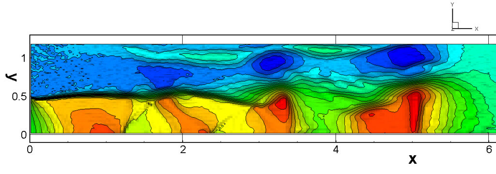
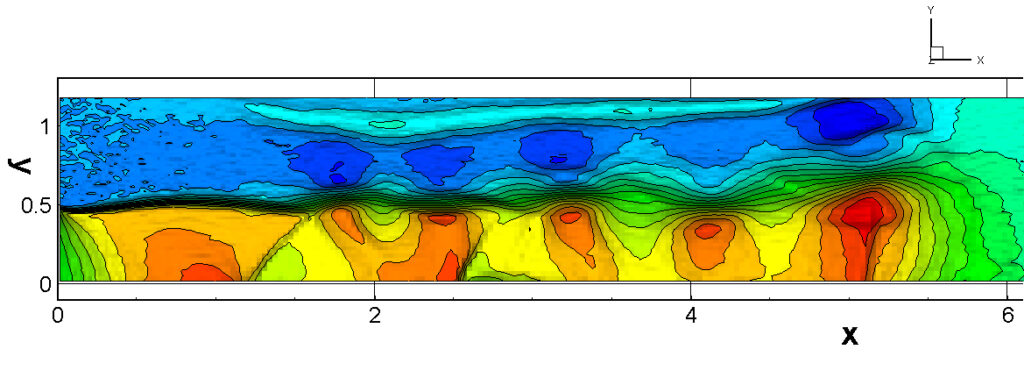
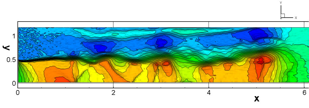
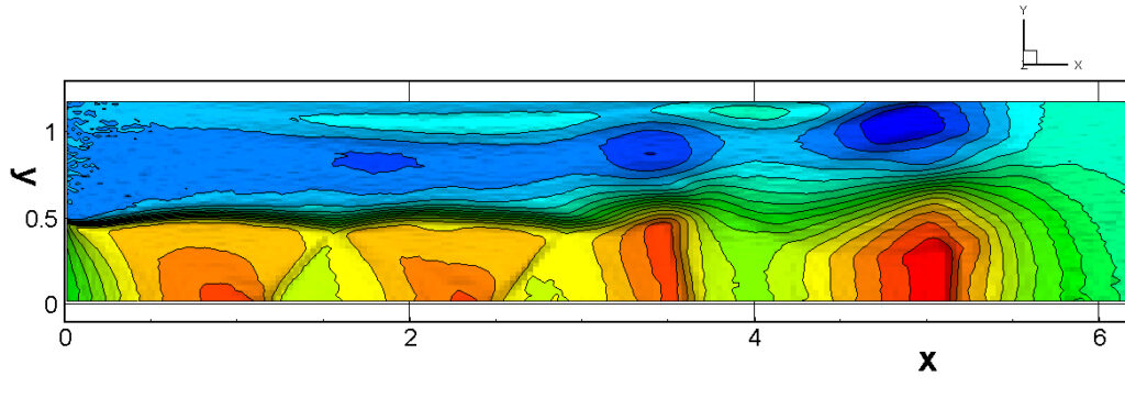
The U-sys method is a method of “predicting and giving the flow velocity and temperature distribution within the cell, and correcting the velocity before and after the collision of two colliding molecules”, which aims to achieve the same effect as making the cell smaller even if the spatial cell is large. However, since the flow velocity and temperature within the cell can only be obtained after the calculation is completed, they must be predicted in some way. Since the DSMC method is basically a unsteady calculation, the easiest way to predict is to use the flow velocity and temperature data from the previous time step. However, if the unsteady change is large, it will naturally result in a calculation error. To prevent this, the time step is made small, but this reduces the number of sample molecules, which in turn generates errors. The next method that can be considered is to predict using the data from one and two times before, but if the prediction formula is incorrect, the calculation may become unstable. A safe method is to perform a provisional calculation using the previous data and then use the result to perform the actual calculation, but this will definitely require twice the calculation time. In the calculation example introduced below, as above mentioned, (1) basic method, (2) time step 1/2, (3) time step 1/4, (4) prediction method using two data, (5) provisional and actual calculation method, and (6) method using provisional and actual calculation with a time step of 1/4 are performed and compared, so please use them as a reference. Each method has its own characteristics, so at this point I cannot judge which one is better. In addition, the U-sys method also uses an approximate calculation called bilinear interpolation, so there may be a need to improve that as well. In the first place, calculations of turbulence should be analyzed as a three-dimensional phenomenon, but they are performed using axisymmetric approximation. Therefore, even if certain parts are made precise, careful consideration must be given to how much meaning this has. I would be very happy if you could come up with a better method.
The output data (9 items) are arranged as follows: x coordinate, y coordinate (r coordinate), number density N, flow velocity u, product of number density and flow velocity N.u, temperature T, x-direction temperature Tx, yz-direction temperature Tyz, and Mach number M. The length is normalized by the diameter of a circular orifice (characteristic length), the velocity is normalized by the most probable molecular thermal speed, and the number density and temperature are normalized by their respective initial values.
●Actual calculation
Below, we will explain the calculation procedure for turbulence analysis of a supersonic jet, but we will proceed assuming that you are familiar with the contents of “2. Test (trial) calculation” and have actually performed that calculation. If you are not, please first perform “2. Test calculation” and check whether you can obtain the results without any trouble. It is also recommended that you have experience with “Simulation of flow velocity profile in a circular tube” described in 3.1 and 3.2, if possible.
(A) Files required for calculation
The five files required for calculation are: ① Calculation software main body (P22-S3.exe), ② Initial value file for 65 random number sequences (ransuuM65), ③ Software to convert primary result files to secondary result files (drawing files) (OUT09B-62S.exe), ④ Software to add and average a series of drawing files after the steady state is achieved (AVE3-JETS.exe), and ⑤ One other file (libiomp5md.dll). These are saved in a single compressed file ‘Supersonic Jet (SS-Jet)’, so after downloading it, unzip it and return it to the five files, just like in “2. Test calculation“. A folder called SS-Jet will be created in the download folder or on the desktop, and the five files will be inside it, so run P22-S3.exe. If Microsoft Defender SmartScreen displays a message stating “SmartScreen is unavailable” when you attempt to run the program, simply ignore it—SmartScreen isn’t actually that smart—and proceed by selecting “Run.” Or, If the message “Windows protected your PC” appears, please click “More info” and select “Run” on the next screen. Note that the command prompt screen where the calculation is performed will be easier to see if you set the window width in the properties to 150 or more.

(B) Starting the calculation (entering multiple data from the keyboard)
① Start the calculation software (P22-S3.exe) in the same way as in “2. Test calculation“, and enter 0 for the first calculation or 1 for continued calculation. For continued calculation, files such as uvw333 and tfile2 must already be created. If you select continued calculation, the original calculation conditions (upstream pressure, pressure ratio, calculation method) will be displayed, and if there are no problems, press the Enter key to resume the calculation. If there are problems, press the Ctrl key and C at the same time to interrupt. Note that uvw333 and tfile2 are very large files, so be sure to delete them when you no longer need continued calculation.
②If this is your first calculation, the number of threads on your PC will be displayed. Enter a number equal to or less than this number as the number of threads you will actually use. If a value outside the range of 1 to the maximum value is entered, the maximum value will be selected (the maximum value is the recommended one).
③Enter the upstream stagnation point pressure within the range of 1 to 760 mmHg (Torr). If it is less than 1, it will be limited to 1, and if it is larger than 760, it will be limited to 760.
④Enter the pressure ratio (the ratio of the upstream pressure to the downstream back pressure) within the range of 2 to 16. If it is less than 2, it will be limited to 2, and if it is larger than 16, it will be limited to 16.
⑤Select whether to calculate using the Bird method or the U-system (U-sys method). Basically, we would like you to calculate using the U-sys method, but the Bird method is also included for those who only want to calculate using the Bird method (the Bird method is faster in calculation speed, but you cannot expect very good results).
⑥If you select the U-sys method, you can choose from the following six types of U-sys method, as mentioned above. If you are unsure which one to choose, first choose (1) the basic method. Depending on the pressure and pressure ratio conditions, the calculation is not going well. In that case, please select (1) the basic method.
(1) Basic method, (2) Time step 1/2, (3) Time step 1/4,
(4) Prediction using two data, (5) Temporary and actual calculation method,
(6) Method using temporary and actual calculation with a time step of 1/4
The separation time (minimum time step) between molecular motion and intermolecular collision in the DSMC method is fixed at 0.005 μs this time, so if you output one intermediate result in 200 steps, you will get a calculation result every 1 μs, but if 1/2 time step (100 steps) or 1/4 time step (50 steps), it will be 0.5 μs (100 steps) or 0.25 μs (50 steps). In this case, the number of sample molecules will naturally be reduced, so in order to make the statistical fluctuations the same, two or four consecutive outputs can be combined into one (see following OUT09B-62S.exe), so that, calculation results every 1 μs can be obtained.
⑦Once you have selected either the Bird or U-sys method, the upstream pressure, pressure ratio, and calculation method will be displayed for confirmation. If there are no problems, press the Enter key to start the calculation, and after a few seconds, the calculation will begin for each step. If there are errors, press the Ctrl key and C simultaneously to run the calculation again from the beginning. At the same time as the calculation starts, a file called “Setting Condition” indicating the calculation conditions is created, so its contents will be useful as a record later, but the time the file was created is also valuable as the calculation start time.
(C) Calculation execution status
When a calculation is being executed, it is important to pay attention to how far the calculation has progressed at that point (how many μs have passed since the start of the calculation) and whether the result file is being output smoothly. First, pay attention to the following display on the screen.——————————————————-
@@ PTOR= ….. PRAT= …..
——————————————————-
The first number indicates the upstream pressure, the second the pressure ratio, and the third the calculation method. The third number from the end of that line is the number of threads used in the calculation. Each line from the next indicates first which time step, then the time in μs. However, in the case of the provisional/actual calculation method (Usys5 or Usys6), A (provisional calculation) or B (actual calculation) is displayed at the very top. However, the first result output is only A (provisional calculation). Explanations of other screen notations are omitted here. As the calculation progresses, primary result files named AA04c… are created in the same folder in sequence. At the same time, files such as uvw333 and tfile2 for continued calculations are output.
(D) Secondary result files (drawing files) obtained by OUT09B-62S.exe
The created primary result file (AA04c…) can be rewritten by OUT09B-62S.exe into a secondary result file (DOWN+xxx-yyy) that can be used to plot the results, and can be used to investigate how far the supersonic jet has grown. This rewriting work must be done sequentially, separate from the actual DSMC calculations. The time to end one condition of DSMC calculations must be also determined by plotting the jet structure at each moment.
Start OUT09B-62S.exe and first enter whether the plot data is for gnuplot or tecplot. Next, enter the last three digits (or the last two digits) of the first primary result file to be processed (leading zeros are not necessary), then the number of the last primary result file, and the number of results to be averaged (usually 1 will give results every 1 μs. However, if the time step is 1/2, enter 2, and if the time step is 1/4, enter 4 to give results every 1 μs). Of course, it is possible to obtain results at intervals other than 1 μs. If the average number is other than 1 and the total number of data is not divisible by the average number, an error will occur at the end and the process will be interrupted. If this error does not occur, you can automatically delete the primary result file by entering 1 at the very end, but if the process is interrupted due to an error, the primary result file must be deleted manually. Primary result files are quite large, so be sure to delete them when they are no longer needed and do not let them accumulate unnecessarily.
You can also use AVE3-JETS.exe to average secondary result files (drawing files) to create results averaged over a long period of time. For example, suppose 10 pieces of data have been obtained: DOWN-301-304, DOWN-305-308, ….. , DOWN-337-340. Start the software (AVE3-JETS.exe) to average them, and first input whether the data is for gnuplot or tecplot. Next, input the starting number 301, the width of one data piece 4, and the number of data pieces 10, and a long-term average file will be created with the name 1-AVE==301-340.
As explained in Chapter 3, “Velocity profile in a circular tube,” tecplot, which I use exclusively, has a function to connect each of the result figures in succession to create an animation, but gnuplot does not have this function, so to create an animation from gnuplot results, please find free animation creation software available on the Internet and use it. Finally, I will post some of the results I have calculated so far (You may reproduce the examples without permission, but please cite the source ‘DSMC calculation by M.Usami (https://usamimas.net)’, and the same applies to descriptions in other chapters.). Although all of them require a considerable amount of calculation time, they can be calculated using the software released this time, so please give it a try and compare them. Note that I will not show examples of gnuplot plots here, so please refer to Chapters 2 and 3 for gnuplot plots.
(E) Calculation examples
① p=760mmHg, p_ratio=16, U-sys_1
② p=760mmHg, p_ratio=11, U-sys_1
③ p=760mmHg, p_ratio=7, U-sys_1
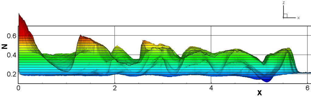
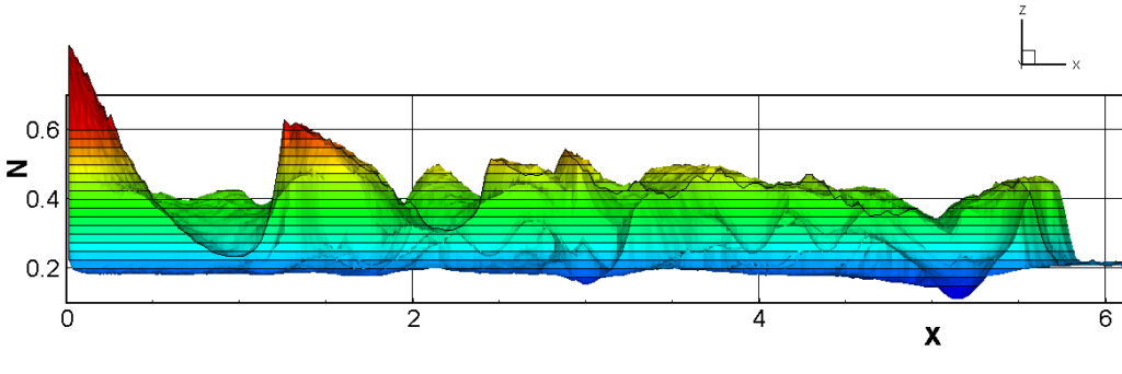
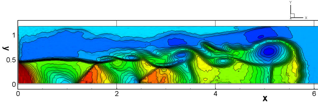
④ p=760mmHg, p_ratio=4, U-sys_1
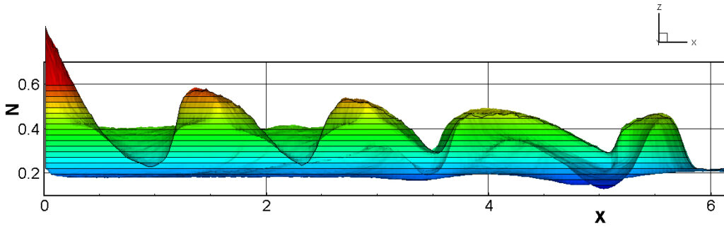
⑤ To compare with Usys1, the results (video) for pressure ratios of 4, calculated using Usys6 (temporary/actual calculation method with time step 1/4), are shown below.
⑥ p=760mmHg, p_ratio=2, U-sys_1
⑦ To compare with Usys1, the results (video) for pressure ratios of 2, calculated using Usys6 (temporary/actual calculation method with time step 1/4), are shown below.
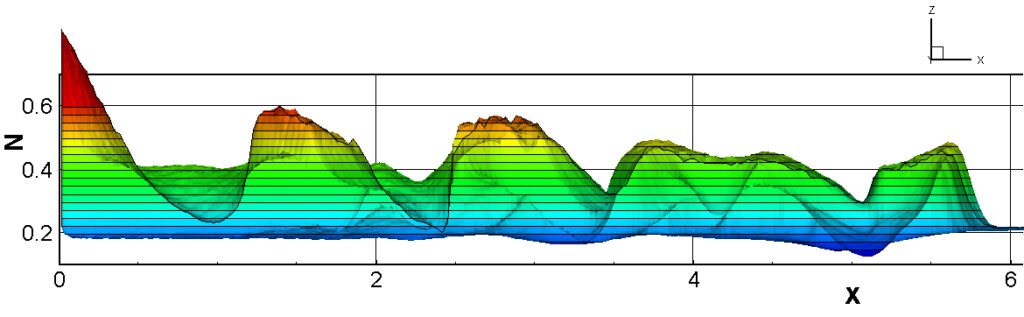
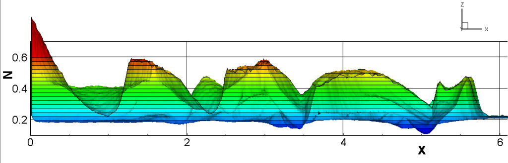
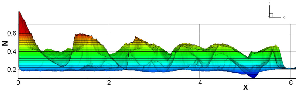
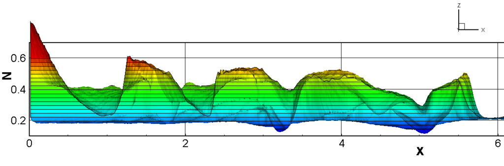
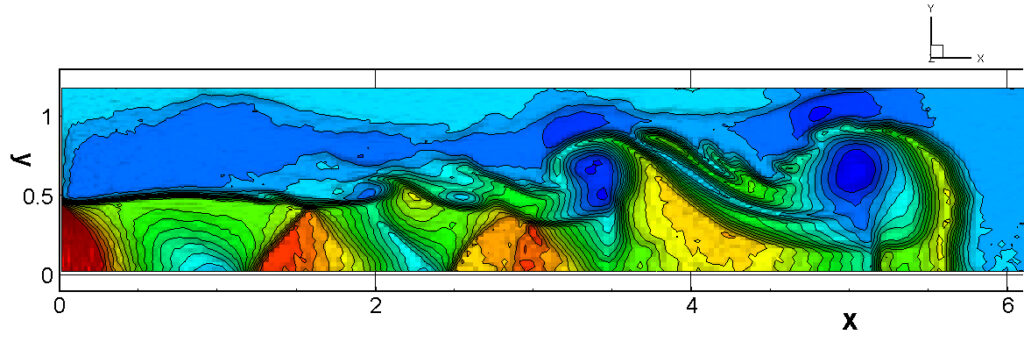
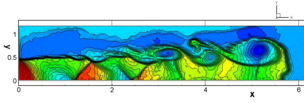
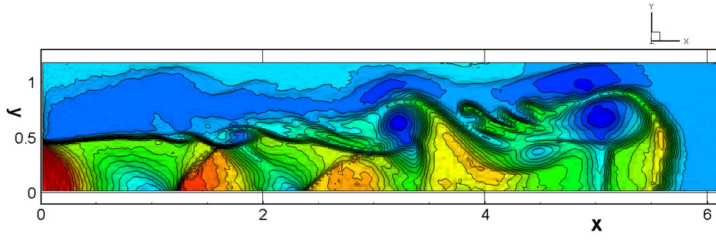
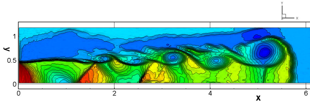
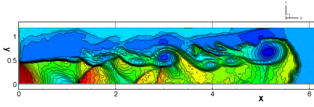
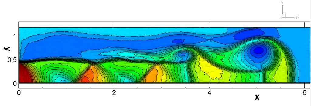
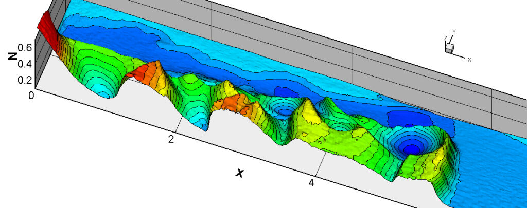
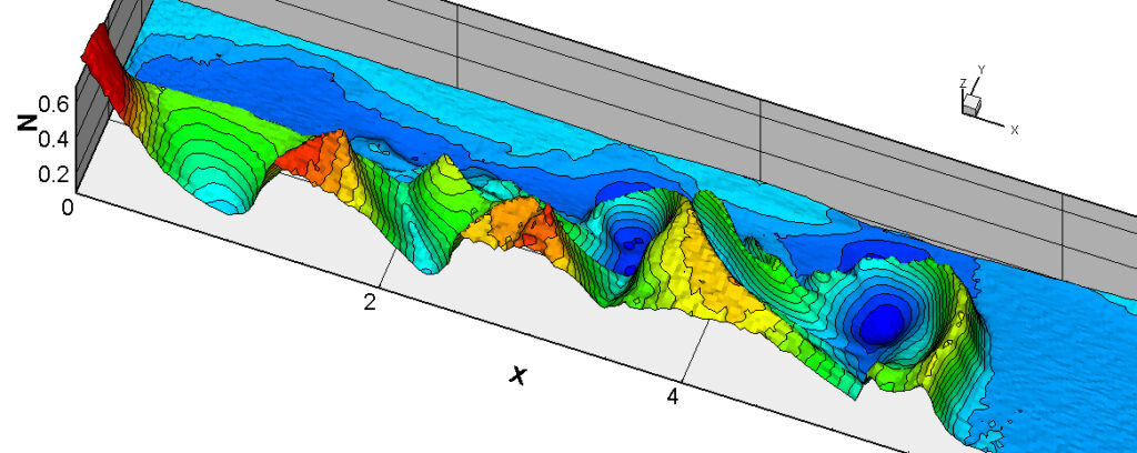
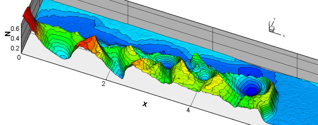
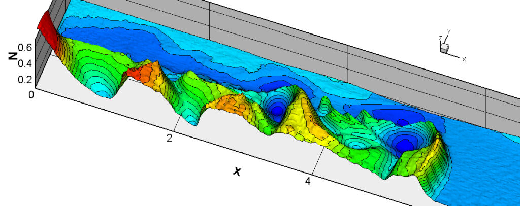
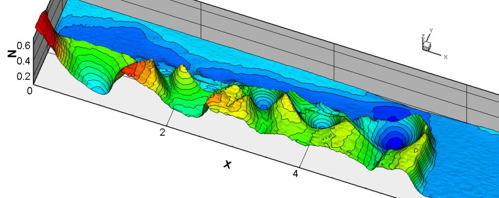
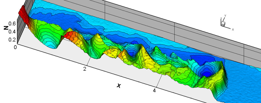
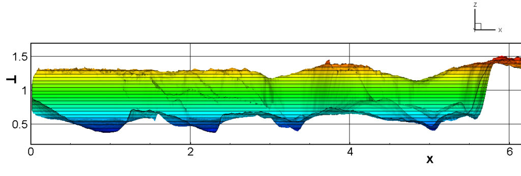
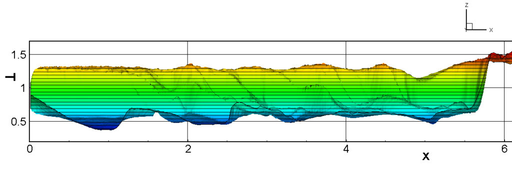
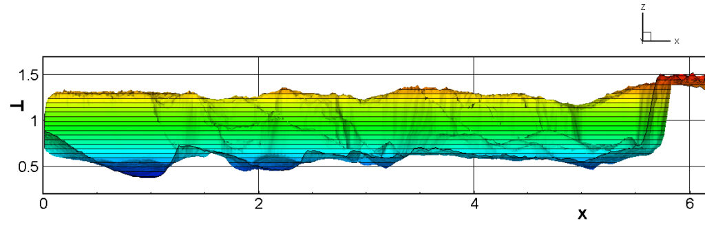
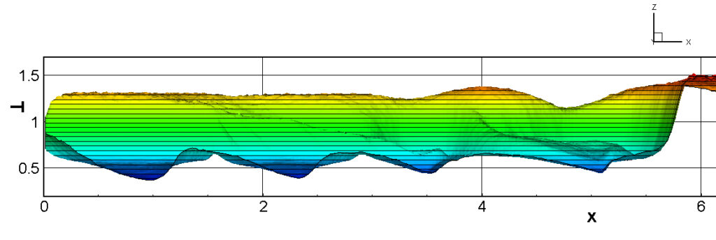
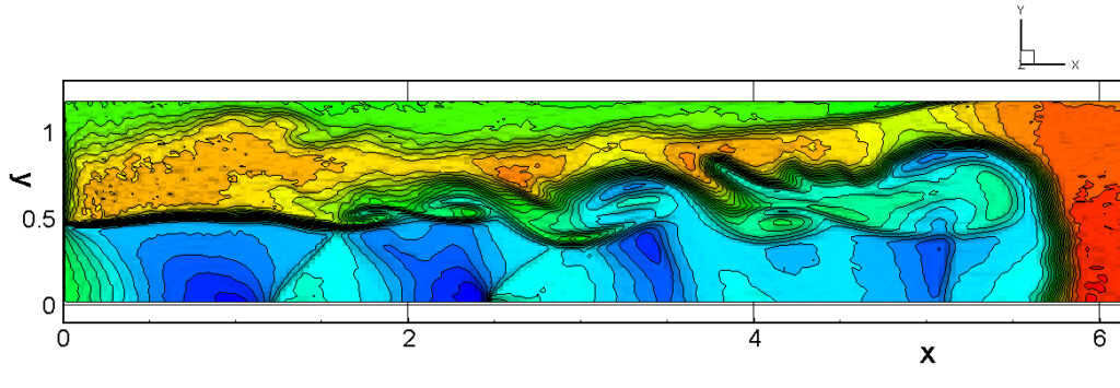
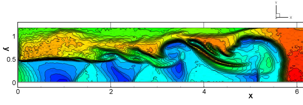
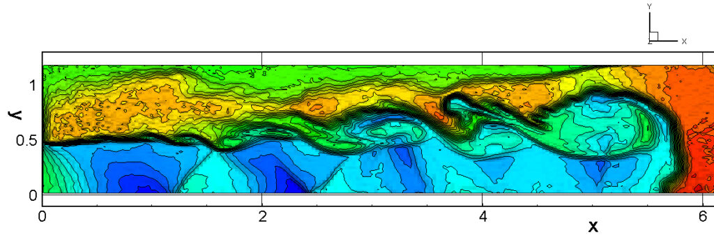
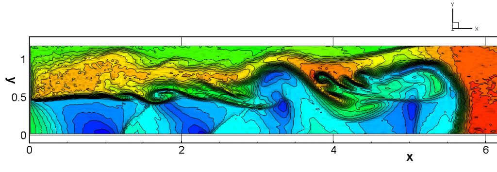
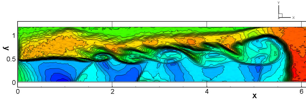
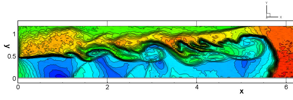
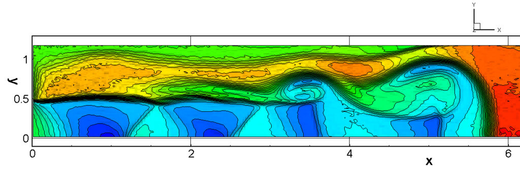
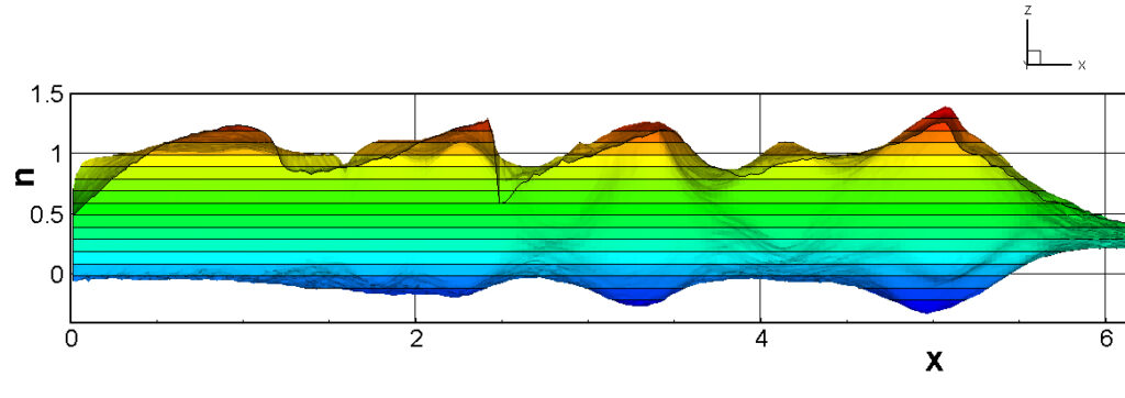
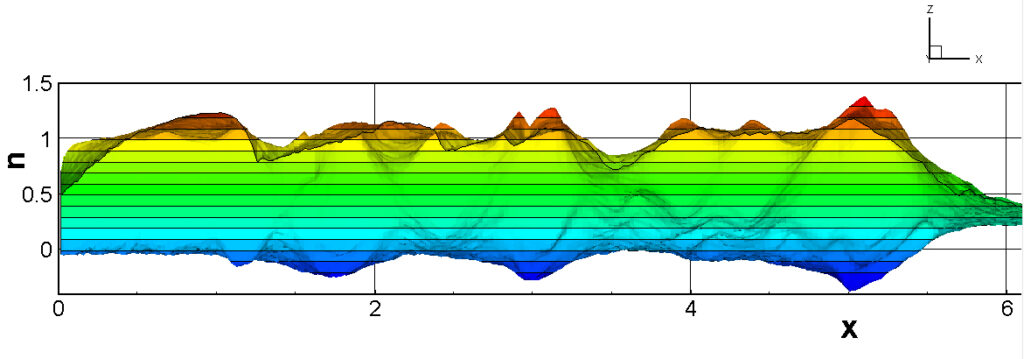
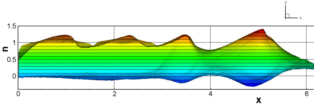
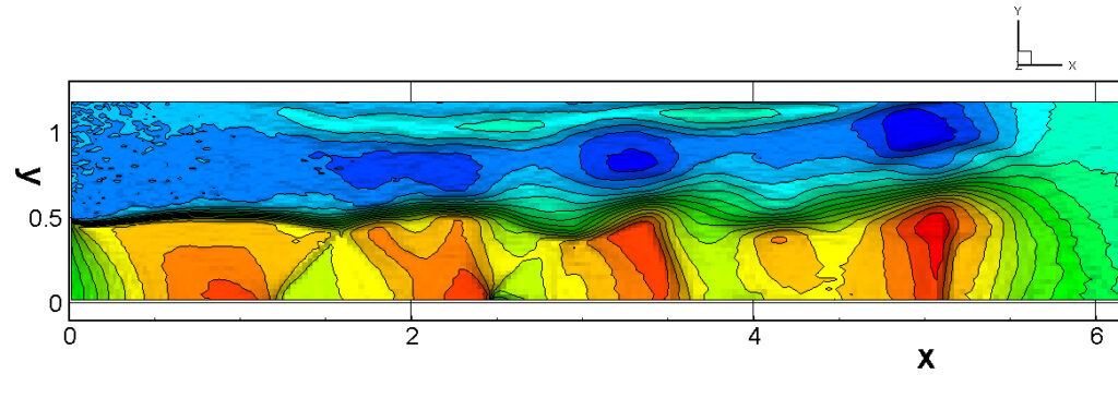
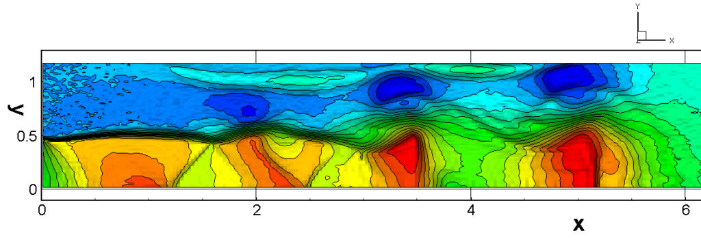
⑧ For comparison, still images obtained at the same time (70μs after the start of jet flow) using different methods with an upstream pressure of 760 mmHg and a pressure ratio of 4 are shown. Each has its own characteristics, and it is not possible to say which is better, so please judge for yourself which is better.