Before providing calculation software for flow velocity distribution in a cylindrical tube, it is important to note several points.
The mechanism for generating the disturbance is to make the wall surface into a saw blade shape and reflect the molecules from it. However, rather than actually making the inner wall uneven, the surface remains flat, and a saw blade shape is apparently used in the axial direction, only to determine the direction in which molecules are reflected. For convenience, this will be referred to as surface roughness from now on (Usami’s surface roughness in the DSMC method). This is what I was referring to when I said “artificial approximation” earlier. Some people may find this difficult to accept, but disturbances originally include such unnaturalness. The unevenness of the saw blade is symmetrical, and the spacing between the saw blades (specifically, the number of blades for a certain length is input) and the angle of the saw blade are specified as a set of parameters. Note that the repeating two or more sets of different parameters can be set along axial direction, but the software in this time is limited to only one set. Since the saw blade is symmetrical and the number of blades is an integer, the force exerted on the wall by the reflective molecules should be zero in a steady state, but in reality, it seems that the force is applied slightly in the opposite direction to the flow, and the flow appears to be slipping a little on the wall.
The flow from the wall toward the center axis (flow in y direction) is stronger on concave surfaces and weaker on convex surfaces, so something similar to Rayleigh-Taylor instability occurs, causing fluctuations in the flow near the wall surface, which becomes a disturbance. In the previous description, it was stated that the axial region length should be greater than or equal to the cylinder diameter. But since periodic boundary conditions are used at the entrance and exit of the circular tube, calculations can be made if you use the length of a few saw blades (the calculation time is approximately proportional to the length). The software provided this time calculates a tube length that is approximately the same length as the diameter of the circular tube (there are some differences in size because the saw blade is an integer). Once a steady state is reached after outputting some intermediate results during the calculation, the calculation continues until a smooth average value is obtained, so it takes a considerable amount of time to complete.
The data to be input is ①the number of threads to use (maximum number is recommended), ②Re number (Input for Re number is limited to 1000 to 7000, because statistical fluctuations become severe when less than 1000, and there is a possibility that compressibility may appeare when more than 7000), ③the number of saw blades (the number of blades can be specified as a real number with a decimal point, in which case the number of blades itself will be rounded off to an integer and then tube length does not necessary match the tube diameter), ④the blade angle (angle from wall surface), ⑤Bird method or U-sys method (U-sys method is recommended), ⑥initial velocity distribution (uniform distribution or parabolic distribution), ⑦calculation from the beginning or continuous calculation, and ⑧whether to output the results for gnuplot or tecplot. You need to decide in advance what you will use. Note that calculations can also be performed without considering surface roughness (smooth surface). If you are doing calculations for the first time, you may be confused about what input data to use regarding surface roughness. So I also propose the values that I currently recommend. If you want to use it for the time being, just input the Re number and you can obtain the recommended value (number of blades and blade angle) in the range of Re = 1000 to 7000. The value introduced by the past experience data for the number of blades and for blade angle in the range of 1000 to 7000 is calculated with a simple function so that 1000<Re<2000 gives a parabolic distribution, 3000<Re<7000 gives a turbulent distribution and 2000<Re<3000 gives transition state. The two calculation formulas written in Fortran code are shown below (‘**‘ is the exponent symbol). For Re, H is the number of blades and K is the angle (degree).
H=(((5000./Re)**3-1.)/15.44+1.)*10.
K=0.111*Re*Re/1000000+1.687*Re/1000+18.26
Although it is easy to use, these two functions are simply mathematical interpolations and have no physical meaning. On the other hand, if the present simulation does have any physical meaning, it will require considerable further investigation and study to clarify this. This is not only my assignment, but also a homework assignment for everyone reading this right now. The average flow velocity changes from 10 m/s to 70 m/s in proportion to the Re number, but since the molecular velocity that is the basis of the calculation is about 350 m/s, the lower the average flow velocity, the more severe the fluctuating components that appear in the results will be. Therefore, the number of samples required to obtain a smooth average value, that is, the number of repetitions of calculation, is required. Possible ways to change the Re number also include changing the density and representative length, but in that case, it is necessary to investigate in detail how the fineness of cells that divide the physical space in DSMC calculations affects the calculation results. Therefore, this time, we will adjust the Re number only by changing the average flow velocity.
The output data sequence (11 data) is x coordinate, y coordinate (r coordinate), number density N, u/U (flow_velocity/average_flow_velocity), flow velocity u, N.u (number_density times flow_velocity), temperature T, x direction temperature Tx, yz direction temperature Tyz, v/U (flow_velocity_v/average_flow_velocity), and flow velocity v. Note that length is normarized by the tube diameter, velocity is normarized by the average flow velocity or by the most probable molecular thermal speed. Number density and temperature are normarized by their initial values respectively.
●● Actual calculation ●●
Below, we will describe the calculation procedure for determining the flow velocity distribution in a cylindrical tube. As a prerequisite for the calculation, we will proceed with the discussion assuming that you are familiar with the contents of “2. Test Calculation” and have actually experienced the calculation. If this is not the case, please run “2. Test Calculation” first and check whether the results are obtained without any problems.
(A) Files required for calculation
The four files required for calculation are: ① Calculation software main body (A-OUT6.exe), ② Initial value file of 65 random number sequences (ransuuM65), ③ Software for averaging a series of result files after steady state is achieved (DATA6-AVE3.exe), and ④One other file (libiomp5md.dll). They are saved in one compressed file ‘Velocity_Profile (VelocityD)’, so just like in “2. Test Calculation” download it and unzip it back into four files. A folder called VelocityD will be created in the download folder or on the desktop, and there will be four files in it, so run A-OUT6.exe. If Microsoft Defender SmartScreen displays a message stating “SmartScreen is unavailable” when you attempt to run the program, simply ignore it—SmartScreen isn’t actually that smart—and proceed by selecting “Run.” Or, If the message “Windows protected your PC” appears, please click “More info” and select “Run” on the next screen. The command prompt screen where calculations are executed will be displayed more easily if you set the window width of the property to 175 or more.

(B) Start calculation (enter multiple data from keyboard)
① Follow the same procedure as in “2. Test Calculation” to start the calculation software (A-OUT6.exe). The number of threads on the PC you are using will be displayed, so enter a number less than or equal to that number as the number of threads actually used. If a number other than 1 to the maximum value is entered, the maximum value will be selected (the recommended value is the maximum value).
②Next, enter 0 for the first calculation, or 1 for continuous calculation. For continuous calculation, files such as uvw333 and tfile2 must already be created.
③Select whether to calculate using Bird method or U-system (U-sys method). Basically, it must be calculated using the U-sys method, and the Bird method is simply included for those who want to make comparisons.
④Enter Re number (1000 to 7000).
⑤ Specify whether the inner wall surface of the cylinder should be a “smooth surface” or a “rough surface.” If a smooth surface is selected, a parabolic distribution of flow velocity will be obtained regardless of the Re number. If you select the rough surface, you will have the choice of determining the two parameters of the saw blade shape yourself or using the recommended values. If you decide on your own, you will need to enter two values, but if you select the recommended value, that value will be displayed and you will move on to the next item.
⑥ Before starting the calculation, select the initial distribution of flow velocity. Select whether to use a uniform distribution with the average flow velocity or a parabolic distribution. If possible, it is better to choose an initial distribution that is different from the final result so that you can observe how the velocity distribution gradually changes.
⑦Select whether to output the results in gnuplot format or tecplot format. The difference between the two result files for gnuplot and tecplot is that the tecplot file has two extra lines at the beginning, so you can change it to the gnuplot file by manually deleting them. Compare the two result files and find out how to make changes on your own.
Once all the above inputs are completed, calculation will start.
(C) State during calculation execution
What you need to be careful about while running a calculation is how far the calculation has progressed at that point, and whether the result file is being output smoothly. First, please pay attention to the following part of the screen display.
——————————————————-
@@ Re = ….. ….. ….. …..
——————————————————-
The first number is Re number, but it may not necessarily match the input Re value completely. This is because the velocity of the molecules is generated using random numbers, so there will be some differences. For the second and subsequent numbers, first understand the following explanation. That mean,
●When the “time step separating molecular motion and intermolecular collision”, which is the minimum time unit of DSMC calculation, is repeated 200 times, one primary result file (AA04cxx) is created. This is repeated many times (the smaller the Re number, the greater the number of repetitions, since the statistical variation depends on the Re number), and the created primary result files are averaged to make two secondary result files. The formar “DOWN+xxx-yyy” is displayed in detail in the axial direction and the latter “DOWN+xxx-yyy-2” is widely averaged. Note that the primary result files created during calculation will be automatically deleted after the secondary result file is made.●
Next to the Re number is a/b (=IOUT1/IOUT0), where “a” indicates the number of the primary result file to be output next. “b” indicates how many times the primary result file must be output to create the secondary result file. When the secondary result file is created, “a” returns to 1. “b” becomes a large number as the Re number becomes small. The next number shows how many time steps have been performed since the start of the calculation, and the next number shows how many primary result files will be created next time. Then, the number of saw blades input (real number), the number of saw blades rounded to an integer, the ratio of tube length to tube diameter changed by converting the saw blades into integers, and the angle of the saw blade (degree), Bird method or U-sys method, along with the initial velocity distribution. Note that almost the same content as this is written to a file called JB-AKTN2-AKTH, and is updated every time the primary result file is created. Note that files such as uvw333 and tfile2, which are created each time a primary result file is created, are necessary to continue the calculation from the middle. If they do not exist in the folder, continuous calculation will not be possible. The other screen displays were used during the program development process, and each has a meaning, but their explanation will be omitted.
(D) Determining whether steady state has been reached and calculating the average of subsequent results
Judging whether the calculation has reached a steady state depends on whether the results obtained subsequently no longer change within the range of statistical fluctuations. So if you want to avoid making judgments based on complicated mathematical formulas, for now, you have no choice but to see it with your own eyes. The only way to do this is to visually compare the resulting diagrams and judge convergence based on experience. In my experience, I think that xxx and yyy in the secondary result files DOWN+xxx-yyy and DOWN+xxx-yyy-2 reach a steady state while varying from 001 to 999 (probably by the 500th time). Note that, after the number 999, the numbers change from 1000 to 2000, but since only 3 digits can be displayed, different symbols can be used to identify them. If it exceeds 2000 times, it will be overwritten with the same name as the first file. A specific example of displaying results using gnuplot will be described later.
Now, for example, suppose that 10 data of DOWN-301-315, DOWN-316-330, ….., DOWN-436-450 were obtained after steady state was achieved. Start the software (DATA6-AVE3.exe) to average them, first input whether the data is for gnuplot or tecplot, then input the starting number 301, the width of one data 15, and the number of data 10. If you will input above data in order, the average for data ‘DOWN+xxx-yyy’ will be created with the name ‘1-AVE==301-450’, and the average for data ‘DOWN+xxx-yyy-2’ will be created with the name ‘2-AVE==301-450’. This allows you to obtain results with less statistical variation.
When using tecplot to display results, it has a function to create an animation by sequentially stitching the resulting figures one by one, but as far as I know, gnuplot does not have that function. Therefore, to create animations with gnuplot, find free animation creation software available on the internet and use it. Finally, I will show two examples of displaying results using gnuplot (plot instructions are displayed below the figure), so please refer to them when plotting the results using gnuplot. Furthermore, ‘set view 90, 90’ or ‘set view 75, 55’ is a command to adjust the viewing angle of the figure.
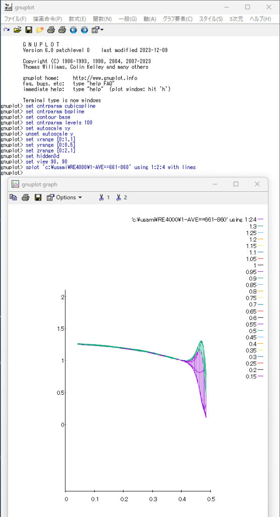
set cntrparam cubicspline
set cntrparam bspline
set contour base
set cntrparam levels 100
set autoscale xy
unset autoscale y
set xrange [0:1.1]
set yrange [0:0.5]
set zrange [0:2.1]
set hidden3d
set view 90, 90
splot ‘c:\usami\RE4000\1-AVE==661-860’ using 1:2:4 with lines
——————————————————————————–
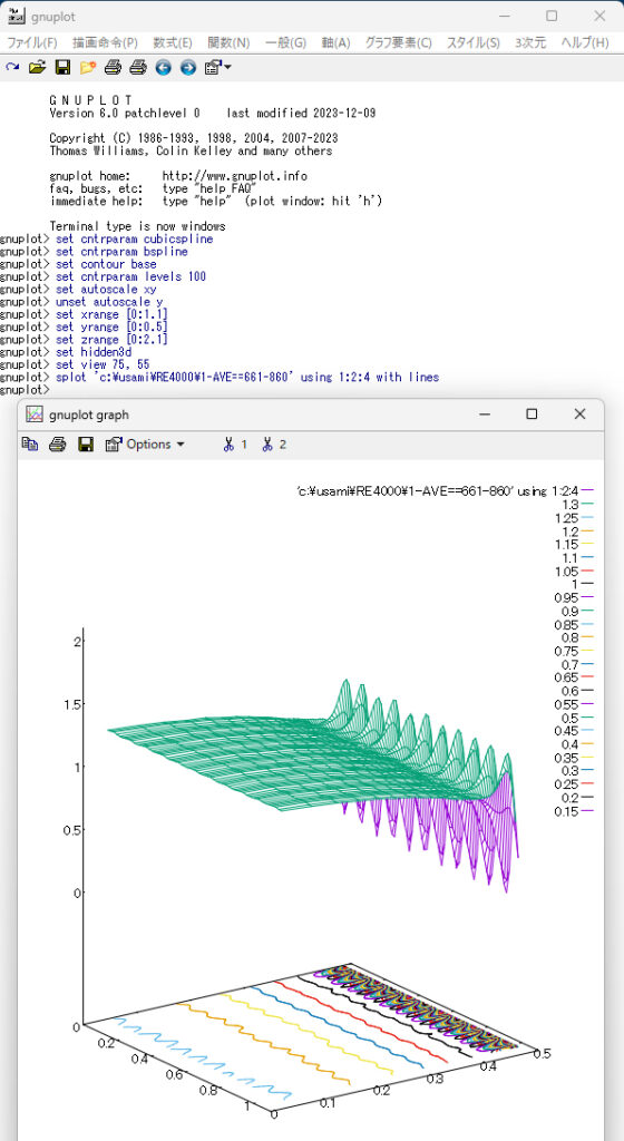
set cntrparam cubicspline
set cntrparam bspline
set contour base
set cntrparam levels 100
set autoscale xy
unset autoscale y
set xrange [0:1.1]
set yrange [0:0.5]
set zrange [0:2.1]
set hidden3d
set view 75, 55
splot ‘c:\usami\RE4000\1-AVE==661-860’ using 1:2:4 with lines
——————————————————————————–
As this is the first time we are releasing this software to the public, I think there may be any flaws. We have set up an “Inquiry column” for you to ask any questions you may have regarding this, so please use it.