In the DSMC calculation in this blog, two methods can be selected: Bird’s original method (Bird method, B_original or B_origin) [Reference 1),2),3)] and Usami’s improved method (Usys method or U_system) including Q.Sun et al.’s proposal [Reference 4),5),6),7),8),9)]. Compared to B_origin, U_system takes more calculation time, but it has the same effect as making the cell finer, and it is effective for calculation in relatively high density condition where it is difficult to adopt a cell length comparable to the mean free path. However, due to the nature of the algorithm, such as using the flow field state before the present time for calculation, there is a lack of theoretical support, and it is not necessarily a method widely accepted by academic societies. Which method you use is up to you. Of course, it is also good to calculate both and compare the superiority and inferiority by yourself. Due to the unique randomness of the Monte Carlo method, which uses random numbers, it is expected that the DSMC method will enable the reproduction of turbulence phenomena. This will be shown in the calculation “DSMC calculation of flow velocity distribution in a circular tube“. It would be my great pleasure if those who were interested in the DSMC method after seeing this blog would contribute to the further development of this calculation method in the future.
Simple calculation of supersonic free jet
After fixing the pressure ratio between upstream and downstream to 50, specify the upstream pressure arbitrarily, and the density, velocity, and temperature profiles of the supersonic jet generated by a single argon gas blowing out from a circular orifice are reproduced by the DSMC method. Axisymmetric is assumed. This time, because of a trial calculation, a very coarse network of spatial cells is used. This is the first DSMC calculation in this blog, so the calculation conditions other than the upstream pressure are fixed and cannot be changed in order not to make a mistake in the operation.
(please note)
This blog administrator is not responsible for any troubles, damages, or proceedings with a third party caused by the execution of the downloaded software. If you disagree with this, please stop the download immediately. If downloaded, it is considered that you have agreed to this.
(A little longer comment)
We recommend the following method to minimize troubles when executing calculations with this software. Of course, you don’t have to do this. It is a precaution just in case.
(1) While the calculation is being executed, the PC would be better off not being connected to the Internet (preferably unplug the network cable).
(2) If something you want to connect to the net occurs during the calculation, you may interrupt the calculation. Since the data in the middle state is recorded occasionally during the calculation execution, the calculation can be restarted later using the data. The same is true for calculations that last for long hours (or days), allowing the PC to rest prematurely.
(3) After completing the calculation, first check the security using reliable security software and check if there is a problem with your PC. It is better to perform the security check without connecting to the internet, but this is not the case if you cannot check without connecting to the internet.

1. Download the compressed file FILE001e and decompress it into three files. Specifically, the downloaded FILE001e.zip will be created in the Downloads folder of your PC, so drag and drop it as it is to the icon of the decompression tool on the desktop installed in advance. As a result, the FILE001e folder is created on the desktop, and three files are created in it. You may execute the calculation in the folder, but in general, make a new folder with an arbitrary name and put three files in it where the simulation is executed.
2. Double-clicking the file JET-P3S2.EXE (or just JET-P3S2) opens a command prompt (black window) in which the calculation starts. If Microsoft Defender SmartScreen displays a message stating “SmartScreen is unavailable” when you attempt to run the program, simply ignore it—SmartScreen isn’t actually that smart—and proceed by selecting “Run.” Or, If the message “Windows protected your PC” appears, please click “More info” and select “Run” on the next screen.
3. Perhaps the command prompt is narrow, so right-click at the top of the command prompt to open Properties and widen the window size in the layout to around 140-150.
4. The following 6 inputs are required at the start of calculation.
(1) Enter the upstream pressure in units of Torr (same as mmHg). For example, enter 760 (atmospheric pressure). As this value is reduced, the structural change of the jet observed becomes weak. It is especially easy to understand when comparing the densities. If you enter a value that exceeds 760 Torr, you will be limited to 760 Torr.
(2) Enter 1 when calculating with Bird_original, or enter 0 when calculating with U_system.
(3) Next, when the message “… OK?” is displayed, usually simply press the Enter key.
If you want to reduce the number of lines displayed during the calculation to about 1/10, enter C or c. Reducing the number of display lines saves some calculation time.
(4) You will be asked whether to execute the calculation (Simulation) or data processing (Data Processing). Enter 0 for the execution of calculation or 1 for the data processing. If the calculation is completed normally, the data processing operation follows automatically.
(5) Since the number of threads of your PC is displayed, enter the number of threads used for calculation by selecting a value between 1 and the displayed (maximum) number of threads (usually, enter the maximum number). If a number outside the range is entered, the maximum number is used. In the case of a PC with multiple CPU chips, in this blog, it is not possible to connect cores and threads of different CPU chips for parallel calculation. Also, due to the restrictions of Windows, parallel calculation exceeding 64 cores or 64 threads is not possible.
(6) You will be asked whether to start the calculation from the beginning (From the Start) or to continue the calculation from the middle of the calculation (Continuation). Enter 0 for the continuation calculation or 1 for the continuation calculation.
(7) When the calculation is completed, the calculation time is shown in seconds as’= Calculation Time (sec)’. Check it and press the Enter key to move to the procedure for processing the result. If the calculation time measured over different months, the correct time may not be displayed.
5. Operation during calculation
(1) Many numerical values appear continuously on the screen as the calculation is executed. In order to know its meaning, it is better to decipher the Fortran source code, but this time we will omit it. If you focus on the number displayed second from the left, you can see that the number increases by 1 (10 when the number of displayed lines is 1/10). This shows how many times the “discrete time step” that separates “molecular motion” and “intermolecular collision” has been counted from the start of the calculation. The intermediate time data of the simulation is saved every 1000 times to allow calculations from the middle, and when this reaches 20000, the calculation ends.
(2) If you want to interrupt the calculation in the middle, you can delete the displayed command prompt (black window) even during the calculation.
6. Result processing
The following three inputs are used during result processing.
(1) Enter 0 for gnuplot or 1 for tecplot as the output data.
The output file names will be Ognu020 or Otec020, respectively.
(2) Enter 0 to set the display result to “data with dimensions”, or enter 1 to set the display result to “non-dimensional data with the upstream value as 1”. Enter 1 usually. The flow velocity is normalized by the most probable molecular thermal speed at the upstream temperature.
(3) Enter the maximum cutoff value in the x-axis (flow direction) of displaying the result. The maximum cutoff value is required because the data near the downstream boundary may be distorted. Normally, about 10 (10 times the orifice diameter) is sufficient, but if you want to know how much the distortion is, enter 15. You can also specify the cutoff value with gnuplot, which will be described later.
(4) After the processing is completed, the value of the upstream pressure is shown for confirmation and the operation is temporarily stopped. When the Enter key is pressed, the command prompt (black window) disappears.
7. How to display the flow field in gnuplot
As for how to use gnuplot, many explanations can be found on the Internet, so I will leave the details to them, but here I will show one concrete example of the result display. For how to use tecplot, please read the instruction manual attached to the software. In the following, the \ symbol cannot be used in Japan, and the ¥ symbol is used instead.
(1) First, launch gnuplot_5.4.
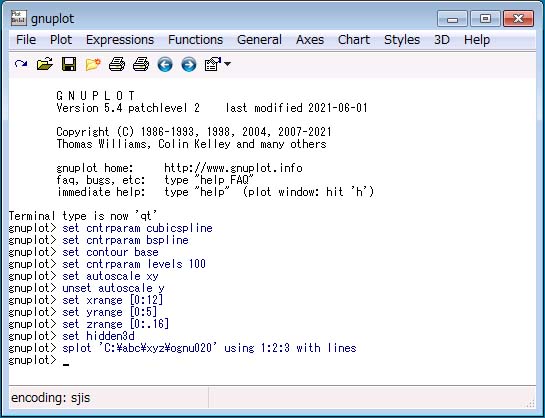
(2) Write the following 11-lines statement in the gnuplot Window. The expression “C:.….” appearing in the 11th line represents the name of the folder containing the file “Ognu020”. For example, if the file “Ognu020” is in the folder “xyz” in the folder “abc” in the C drive, it will be “C:\abc\xyz\Ognu020”.
set cntrparam cubicspline
set cntrparam bspline
set contour base
set cntrparam levels 100
set autoscale xy
unset autoscale y
set xrange [0:12]
set yrange [0:5]
set zrange [0:0.16]
set hidden3d
splot’C:.….\Ognu020′ using 1: 2: 3 with lines
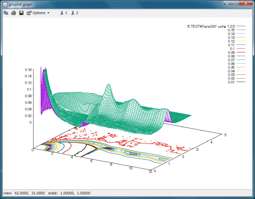
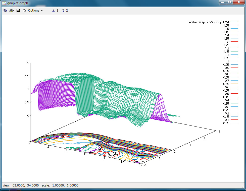
These lines open the window of the gnuplot graph and displays the density profile. Next, if you write the following two lines, the flow velocity profile “u” in the x direction will be displayed.
set zrange [0:2]
splot’C:.….\Ognu020′ using 1: 2: 4 with lines
If you write the following two lines, the flow velocity profile “v” in the y direction will be displayed.
set zrange [-0.5:1.5]
splot’C:.….\Ognu020′ using 1: 2: 5 with lines
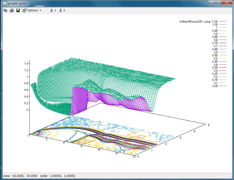
Furthermore, if you write the following two lines, the temperature profile will be displayed.
set zrange [0:1.5]
splot’C:.….\Ognu020′ using 1: 2: 6 with lines
Each displayed graph can be rotated by placing the mouse cursor in the gnuplot graph and then using the mouse or arrow keys. However, since the reaction of this software is very slow, it is necessary to operate the graph movement and rotation slowly. For the instructions on each of the above lines, refer to “Help” in gnuplot.
(Result gnuplot graph) Upstream pressure is 760 Torr, U_system.
(a) Density profile
(b) Flow velocity profile in the x-direction
(c) Temperature profile
8. Some examples of calculation time for ‘JET-P3S1’ by various PCs with multi-core or multi-thread processor.
Upstream pressure is 760 Torr, U_system, and the maximum number of threads for each CPU is used. Since this is a small-scale calculation, this tendency does not necessarily apply to large-scale calculations. There is a difference of about 100 sec depending on the number of lines output during the calculation. Depending on whether the recording medium is an HDD or SSD, or M.2 SSD, as well as the type (SATA, NVMe) and the release generation, since the writing speed differs greatly of a large amount of intermediate data to be recorded for continuation calculation, the ending time is also affected by these differences. If your PC is significantly slower than the example below, the BIOS and/or msconfig may have limited the number of threads available and you need to remove that limit.
(1) Tablet PC (Win10) CPU: Celeron-N4120 (4 cores) 4348 sec
(2) 14-inch notebook (laptop) PC (Win7) CPU: i7-3517U (4 threads) 4389 sec
(3) 13-inch notebook PC (Win7) CPU: i7-4510U (4 threads) 4445 sec
(4) 17-inch notebook PC (Win7) CPU: i7-2860QM (8 threads) 2633 sec
(5) 14-inch notebook PC (Win11) CPU: i5-1235U (12 threads) 1656 sec (I asked my acquaintance who has this PC to measure the calculation time)
(6) 16-inch notebook PC (Win11) CPU: AMD-6800H (16 threads) 791 sec
(7) Desktop PC (Win7) CPU: Xeon E3-1280 V2 (8 threads) 1604 sec
(8) Desktop PC (Win10) CPU: Xeon E5-2699 V3 (36 threads) 693 sec
(9) Desktop PC (Win10) CPU: AMD-2990wx (64 threads) 500 sec
(10) Desktop PC (Win10) CPU: AMD-3970x (64 threads) 366 sec
(11) Desktop PC (Win10) CPU: AMD-3990x (64 cores) 302 sec
(64 threads, if 64 threads of another group is not working) 374 sec
(64 threads, if 64 threads of another group is being used to do another job) 404 sec
(128 threads) Not executed because a large program rewrite is required due to Windows restrictions.